A Simplified Approach to Multivariable Model Predictive Control
Michael Short
1,*1Electronics & Control group, Teesside University, Middlesbrough, UK.
Received 27 May 2014; received in revised form 05 December 2014; accepted 09 December 2014.
Abstract
The benefits of applying the range of technologies generally known as Model Predictive Control (MPC) to the
control of industrial processes have been well documented in recent years. One of the principal drawbacks to MPC
schemes are the relatively high on-line computational burdens when used with adaptive, constrained and/or
multivariable processes, which has warranted some researchers and practitioners to seek simplified approaches for
its implementation. To date, several schemes have been proposed based around a simplified 1-norm formulation of
multivariable MPC, which is solved online using the simplex algorithm in both the unconstrained and constrained
cases. In this paper a 2-norm approach to simplified multivariable MPC is formulated, which is solved online using a
vector-matrix product or a simple iterative coordinate descent algorithm for the unconstrained and constrained cases
respectively. A CARIMA model is employed to ensure offset-free control, and a simple scheme to produce the
optimal predictions is described. A small simulation study and further discussions help to illustrate that this quadratic
formulation performs well and can be considered a useful adjunct to its linear counterpart, and still retains the
beneficial features such as ease of computer-based implementation.
Keywords: Real-time and embedded control, predictive control, multivariable control.
1.
Introduction
Model Predictive Control (MPC) schemes employ dynamic models of a process in conjunction with on-line optimization
schemes to compute an optimal sequence of input moves which minimizes the predicted future values of an objective function
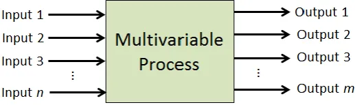
[1][2]. The principal components of most MPC implementations are as shown in Fig. 1. The potential benefits of applying
MPC strategies to complex industrial processes has been well documented in recent years, and includes the ability to deal with
large time delays, non-minimum phase (inverse response) behaviors, and tightly-coupled multivariable systems [1]. MPC is a
form of receding-horizon optimal control, and provides a large amount of flexibility when compared to traditional control
schemes such as pole-placement [16][20]. However one of its principal drawbacks has been the relatively high on-line
computational burden when used with adaptive and/or multivariable schemes [1][2]. This has warranted some researchers and
practitioners to seek simplified approaches for its implementation. Although most modern MPC schemes utilize quadratic
(2-norm) objective functions which are solved on-line by Quadratic Programming (QP) software, much of the original work on
MPC algorithms utilized linear (1-norm) objective functions which were solved on-line by Linear Programming (LP) software
such as the well-known Simplex algorithm [1][3]. This transition is due to several factors, principally due to advances in QP
solving techniques and a number of well-documented drawbacks to the use of LP formulations in MPC. The drawbacks
include possible idle/deadbeat dichotomous behaviors [3], the need to use iterative schemes to obtain solutions even in the
unconstrained case [1][3], and potentially poor scaling in the size of the MPC problem to the corresponding LP [4]. Despite this,
it has been argued that in some situations LP-based MPC may still be effective [3].
*Corresponding author. E-mail address: [email protected]
Fig. 1 Main elements of an MPC strategy
One such situation has received considerable attention in recent years, this is the Simplified Predictive Control (SPC)
technique first described by Gupta [4]. In this approach, a number of simplifications are made to an LP formulation of an MPC
instance with the main aim of reducing the run-time complexity, and also to allow an easier implementation. The
simplifications proposed in SPC are such that the impact on control loop performance is minimal. Although principally aimed
at multivariable MPC, the SPC technique can also be applied to single variable control; as was shown in [8], the performance
of single-variable SPC can be made identical to a well-conditioned Dynamic Matrix Control (DMC) implementation. The SPC
approach has been successfully applied in industry [5] and various extensions have been reported [6], along with favorable
experimental comparisons to other MPC approaches [7] and analytical studies [8]. However, SPC also has several notable
drawbacks. In this paper it will be argued that as with other MPC strategies, the adoption of a 2-norm objective function in SPC
retains much of its beneficial properties and also has the ability to overcome some of the drawbacks. A small simulation study
and further discussions help to illustrate that this quadratic formulation performs well and can be considered a useful adjunct to
its linear counterpart, and still retains the beneficial features such as ease of computer-based implementation. The remainder of
this paper is organized as follows. Section 2 describes the SPC approach in more detail and outlines the nature of its potential
drawbacks. In Section 3, the QP formulation - SPC2 - is introduced and a simple algorithm is presented to obtain optimal output predictions. In Section 4, a simple iterative algorithm is presented to solve constrained SPC2 problems. Section 5 presents a small simulation study to provide an initial validation of the behavior of the proposed approach, and the paper is concluded in
Section 6.
2.
Simplified Multivariable MPC
Consider a potentially over-actuated Multi-Input Multi Output (MIMO) industrial process, such as the one depicted in
Fig. 2, which has a number of interacting control loops featuring m > 1 controlled (output) variables and n ≥ m manipulated
(input) variables. Such a process may be represented as an m-by-n matrix of transfer functions [1][2]. The SPC approach to
control of this process is to select, for each of the m outputs under control, a single point pisteps ahead on the prediction horizon at which the error is to be minimized. For each manipulated variable j, only a single control move ujk is calculated and
applied at the current step discrete k, such that the vector of predicted future errors is minimized.
The pi values thus become tuning parameters, and by increasing (decreasing) their values, a slower (faster) response can
be achieved in each loop in a similar fashion to the use of move suppression co-efficients in regular MPC strategies such as
DMC and Generalized predictive Control (GPC) [4][5][7]. Choice of the pi values cannot be made arbitrarily, they must be
chosen such that they are greater than the time delay and/or inverse response of process loop i in order to prevent instability [4][8]. Prior to the calculation of the control moves at step k, the predicted error in each loop pi steps into the future can be obtained by subtracting the predicted output of the process from the future reference:
i i
i k p
i p k i p k
i
r
y
e
ˆ
(1)Where ŷik+pi is an optimal prediction of the free response of output yi, assuming the previously applied control signal vector uk-1is held constant. If the future reference value ri
k+pi
is not known, then it can be assumed that the current set point
signal rik is held constant over the prediction horizon. In the original SPC approach, a step response model is used to obtain the
predicted free response of the process in a similar fashion to the DMC algorithm [4]. Let the predicted change in output j at pj
steps ahead due to a step change in input ui be given by the step co-efficient gij, which can be obtained with knowledge of the
process transfer function matrix. Then by appropriate manipulations to the n process inputs, the predicted p–step ahead errors
can be minimized for each loop. Thus, once the free errors for each loop have been obtained at step k, a constrained linear optimization problem is then required to be solved:
;
;
:
to
subject
:
respect to
with
:
minimize
max min max min 1e
u
G
e
u
u
u
u
e
u
G
(2)Where u is the n-vector of applied incremental control moves (i.e. uk= uk-1+uk), e is the m-vector of predicted future errors, umax and umin are n–vectors representing lower and upper bounds on the allowed control moves, emax and emin are m– vectors representing lower and upper bounds on the allowed errors, and G is an m-by-n matrix of p-step ahead coefficients:
nm n n m mg
g
g
g
g
g
g
g
g
G
2 1 2 22 21 1 12 11 (3)Although input rate-of-change (velocity) limits and output error constraints are seemingly only present in the constraints
defined in equation (2), due to the simplified nature of the problem position and output constraints can be explicitly enforced at
each step as follows. Suppose the lower and upper actuator and output position constraints are denoted by umin, umax , ymin and
ymax respectively. At iteration k, if the constraints for (2) are first updated according to (4), then these additional constraints will also be enforced by its solution:
Note that as with all constrained MPC approaches, there may be situations in which both the input and error constraints
may not be simultaneously satisfied, in other words (2) is infeasible [1][2]. To overcome this problem, it is common to drop the
error constraints in (2) and consider only rate and position constraints on the input, and set warning alarms should the future
output trajectory be predicted to deviate from its bounds [2][4][9]. This results in a simplified LP formulation with V = 2m + 2n
variables and C = n + m constraints [3]. The SPC algorithm described above has many attractive features compared to regular
multivariable MPC schemes, principally with reduced on-line computation times and easier implementation. In terms of
potential performance reduction due to the minimization of only a single point on the future trajectory, as noted in [4] this loss
of performance should be minimal, as each point on the trajectory is still optimized, but only one step at a time. However, it
also has several notable drawbacks, including:
(i) Even in the absence of constraints, there is no analytical solution to (2) and an iterative solution such as the Simplex
algorithm must therefore be employed; (ii) In order to achieve robust behavior, the pi points may have to be projected a large
distance into the future, which reduces the quality of the output predictions and (iii) Small changes in the predicted future
errors can cause large changes in the applied control signals between iterations k and k+1, as the controls are discontinuously
mapped to the errors due to the use of the least absolute deviations (1-norm) objective function.
All of these points may be problematic in terms of real-time control implementations with embedded processing systems.
The first point may be problematic as control systems, by definition, are real-time in nature and many have hard timing
constraints; in these situations, worst-case behavior in terms of execution time must be taken into account when deciding if the
application software is schedulable on the current computing platform [10]. Although the average-case time complexity of the
simplex algorithm (and its known variants) requires approximately [C+V]3 operations - which is cubic in the number of variables and constraints - its worst-case run-time complexity is O(2[C+V]) and hence exponential [11]. As this potential for occasional exponential behavior must surely be accounted for, in a dependable design the computing platform will be
potentially under-utilized for much of its lifetime [10]. Note that the reliability and stability of the run-time computations
required for most constrained MPC implementations is problematic generally, and is considered to be a major obstacle and an
area of much-needed research [2]. In the regular SPC approach, this problem also applies equally to the unconstrained problem.
The second point can lead to a loss of performance, especially in cases when the system is subject to unmeasured
disturbances and model-process mismatch, which is to be expected in most industrial implementations [1][2]. As noted in [1],
it is impossible to completely prevent noise entering a system and affecting future process predictions, and hence there is no
advantage to be gained in selecting the start of the prediction horizon beyond the process time delay d as the quality of the output predictions decreases. For SPC to be effective in many cases, it must be set well-beyond this lower bound in order to
obtain a robust response [4][5][8]. However, when optimizing only a single error on the predicted output trajectory, as
mentioned above care must also be taken for loops exhibiting inverse responses, regardless of the way the objective function is
formulated: original formulations of the Minimum Variance (MV) control laws also suffered instability problems when
optimizing only a single point d+1 steps into the future, despite the use of a quadratic loss function [19].
The final point can result in ‘chattering’ of the actuators, i.e. large input changes occurring due to small changes in the
predicted errors [3][11]. This can be especially problematic in systems with an ill-conditioned G matrix, and will require the
addition of control signal penalties into the objective function, thus increasing the number of variables in the LP formulation
and increasing computational demand further. The points listed above warrant the search for an SPC algorithm that retains
much of the beneficial properties as the original, but also with the ability to overcome the highlighted problems. Such an
3.
A 2-Norm Approach to Simplified Multivariable MPC
As may be expected, many features of the proposed 2-norm approach to SPC deliberately remain identical to the original
formulation. Again a single point pisteps ahead on the prediction horizon is selected for error minimization, only a single control move for each input is calculated, and only rate constraints (plus position constraints via. (4)) on the input are
considered. A discrete transfer function model with an input disturbance is used to obtain the predicted free responses (and
hence the errors via equation (1)). A simple procedure for calculating predictions is described later in this Section. The main
difference in the formulation of the 2-norm SPC technique (SPC2) is the use of a quadratic objective function, which has many associated benefits which are recapped below:
(i) The use of 2-norm objective function allows for an analytical Least Squares (LS) solution to obtain the optimal
control moves in the absence of constraints; (ii) Regularization (move suppression) parameters can be easily added into the LS
objective function, loosening the dependence between loop robustness and the future prediction point (pi) values, allowing
them to be potentially reduced and temporarily nearer (improved) predictions used, and (iii) The LS approach is stable in that
smooth changes in the future predicted errors result in only smooth changes in the control variables, which are continuous
functions of the errors.
The constrained case reduces to a relatively simple ‘box’ constrained LS problem with no more than n constraints, for
which a simple iterative solver is developed in Section 4.
3.1. Unconstrained case
For the unconstrained case, replacing the objective function of (2) with its 2-norm equivalent and adding regularization
parameters to provide a weighted penalty on the size of the output control moves gives the following simple optimization
problem to be solved at each step k:
u
u
diag
e
u
G
:
respect to
with
)
(
:
minimize
22
22(5)
Where u, l, u, e and G are as previously defined, and is an n-vector of regularization (move suppression) parameters such that each i ≥ 0, 1 ≤ i ≤ n. Note that without loss of generality, a squared 2-norm objective is employed in (5) as the regularization parameters are dimensionless. Clearly, (5) is a simple regularized LS problem; it is a special case of the
multivariable Generalized Predictive Control (GPC) scheme (described in, for example, [1]) featuring only a single point on
the prediction horizon to be optimized per output. Minimization of (5) leads to the following analytical solution to obtain u:
G
G
diag
G
e
u
(
T)
(
)
1 T
(6)The control matrix C = (GTG+diag()) may be easily inverted (or Cholesky factorized into C = LLT) off-line during the design stage [13][14], once the move suppression parameters and pi points have been chosen. At each time step k, once the predicted error vector e has been determined, the optimal control moves can be determined in O(n2) with a simple matrix-vector multiplication or solution via the Cholesky triangle [12][13][14]. Equation (6) may be interpreted as a
state-feedforward control law, in which the current controls are determined as affine functions of the predicted future errors.
Note that as mentioned above, the 1-norm objective function defined by equation (2) has no analytical (closed-form) solution
that can be directly expressed in a form similar to equation (6). Online optimization is required for the solution of (2), and
hence an analytical comparison of the control laws in the unconstrained cases is difficult to perform. In the case where is
embedded systems, as in the worst-case if each element of the vector changes simultaneously, this a full-rank update of C and hence a full rank correction to C-1 is required. However, under the (not unreasonable) assumption that at every time step, only a single element of is likely to change, then the technique of [15] may be employed to efficiently update C-1. Assuming that the kth element of changes by an amount k, then C-1 may be efficiently updated according to:
k kk k kj ik ij
c
c
c
c
1 1 1 11
(7)Where cij (cij-1) is the element corresponding to the ith row and jth column of C (C-1). Computation of (7) may clearly be performed online with complexity O(n2).
3.2. Constrained case
In the constrained case, the following ‘box’ constrained quadratic program is required to be solved at each step k:
max min 2 2 2 2
:
to
subject
:
respect to
with
)
(
:
minimize
u
u
u
u
u
diag
e
u
G
(8)There are several ways to obtain a valid vector of control moves satisfying the constraints in (8), but there is only one
optimal vector [12]. The simplest way to obtain a solution is to ‘clip’ the unconstrained solution; although this works well some of the time, it can on occasion be arbitrarily far from optimality. In Section IV, a simple iterative algorithm for the solution of
(8) will be described.
3.3. Prediction Model
Consider again the multivariable process depicted in Fig. 2. The input/output relationships of the continuous-time
dynamics may be expressed in matrix form as:
)
(
)
(
)
(
s
G
s
U
s
Y
p (9)where:
)
(
)
(
)
(
)
(
,
)
(
)
(
)
(
)
(
)
(
)
(
)
(
)
(
)
(
)
(
,
)
(
)
(
)
(
)
(
2 1 2 1 2 22 21 1 12 11 2 1s
U
s
U
s
U
s
U
s
G
s
G
s
G
s
G
s
G
s
G
s
G
s
G
s
G
s
G
s
Y
s
Y
s
Y
s
Y
n nm n n m m p m
(10)Assuming a Zero-Order-Hold on the inputs and taking z-transforms gives:
)
(
)
(
)
(
z
G
z
U
z
Y
p (11) ) ( ) ( ) ( ) ( , ) ( ) ( ) ( ) ( ) ( ) ( ) ( ) ( ) ( ) ( , ) ( ) ( ) ( ) ( 2 1 2 1 2 22 21 1 12 11 2 1 z U z U z U z U z G z G z G z G z G z G z G z G z G z G z Y z Y z Y z Y n nm n n m m p m (12)
A matrix factorization (e.g. using a left co-prime representation) of Gp(z) into Gp(z) = A-1(z)B(z) allows (11) to be re-written as:
)
(
)
(
)
(
)
(
z
Y
z
B
z
U
z
A
(13)Adding a disturbance model consisting of an integrated white sequence w(k) with zero mean and finite variance gives the
multivariable Controlled Auto-Regressive Integrated Moving Average (CARIMA) model commonly used in GPC [1]:
) ( ) ( ) ( ) ( ) ( )
(zY z B zU z I z W z
A
(14)
Where = 1-z-1 is the difference (delta) operator and I is an n-by-n identity matrix. The advantage of using the model (14) is that the closed loop response will contain an integrator. To obtain an output predictor from (14), first multiply throughout by
to give:
)
(
)
(
)
(
)
(
)
(
)
(
z
Y
z
B
z
U
z
I
z
W
z
A
(15)The usual procedure for obtaining free response predictions using (15) is to employ Diophantine recursions [1].
However, a simplified recursive procedure for predicting the process free response is now described. At discrete time step k, it
can be observed that the expected future values of the random disturbance term w(k+i) = 0 for all i > 0, and since the free response is required, it can be also be assumed that the future controls u(k+i) = 0 for all i > 0. Hence the predicted change in any output j, ŷj(k+1), is trivially obtained from (15) using knowledge of the (known) previous input/output increments y and
u. Similarly, one may easily obtain ŷj(k+2) recursively, replacing yj(k+1) with ŷj(k+1) as required, and then ŷj(k+3), and so on until ŷj(k+pj) is reached. Obtaining the required p-step ahead output prediction ŷj(k+pj) is then trivially achieved through integration:
pj
l j j
j
j k p y k y k l
y 1 ) ( ˆ ) ( ) ( ˆ (16)
This can be easily programmed onto a microcomputer and does not require the use of Diophantine recursions or
specialized software. Finally, note that if the disturbance terms are correlated, a coloring polynomial C(z) may be used in (14)
instead of the identity matrix I. In this case the terms of C(z) may be absorbed into the (suitably expanded) A(z) and B(z) polynomial matrices [1], and the method outlined above applied thereafter. This is perhaps only useful in the adaptive case,
since the terms of C(z) are very difficult to identify and in most cases time-varying [16].
3.4. Parameter Tuning
stable processes. Suppose that the combined process dead-time and inverse response contribution for loop i is di sample times, and the open-loop 95% settling time for loop i is approximately si sample times. Initial simulations suggest that selection of pi
(di, si/2] will give adequate results. With these values selected, then a value for each parameter i is required. Initial experience suggests that they should be selected such that the control matrix C is well-conditioned, with a reciprocal condition
number that is approximately 0.1 to ensure smooth control actions and less sensitivity to noise. The move suppression coefficients can then be adjusted through further simulation to produce the desired performance as needed before application to
the real plant.
4.
Reduced Complexity QP Algorithm for SPC
2The constrained QP technique described in the previous Section has several attractive features as the constraints are only
applied to the inputs, leading to a ‘box-constrained’ least squares optimization problem. Several techniques are known to be
effective in this situation, the most efficient of which are based around ‘active set’ techniques [1][17]. Active set algorithms
operate around the same basic principle, in that constraints which are active at the current iteration are treated as equality
constraints, and the remaining constraints are disregarded. The ‘free’ variables are then solved using standard LS techniques.
Once a minimum to this reduced problem is found, if the solution satisfies the constraints then the Karush-Kuhn-Tucker (KKT)
conditions can be checked to test the optimality of the solution. If the solution does not satisfy the constraints, then one or more
constraints are added into the ‘working set’ and the next iteration is started. If the current solution satisfies the conditions of (9),
then the solution is optimal and the search terminates; otherwise, an active constraint is removed from the working set and the
next iteration starts. For the problem given in (8), if J is the value of the objective function at the current solution point, the KKT conditions reduce to checking the following conditions:
max min
max min
, 0
, 0
, 0
j j i
j j i
j j j
i
u u u
J
u u u
J
u u u
u J
(17)
In other words, moving a variable away from its current position in a valid area of the solution space can only increase
the value of the objective function. Given a candidate solution vector u’, the vector of partial derivatives J required for checking (17) can be computed as J = (GTe) – C-1u’, where C-1 is the inverse control matrix as described in the previous Section. Assuming one is willing to implement a full active set solver and solve up to 2n-1 sets of linear equations at each
sample step, then the active set algorithm developed by Schofield [17] is a good choice. However motivated by the need for
implementation simplicity, in this paper an alternative simple iterative solution based upon coordinate descent will be
suggested. For the problem described in (8), given an initial (feasible) solution u0 and desired optimal solution u*, one may proceed to iteratively generate a series of improved controls u1, u2, u3, … which improve the objective function at each iteration. For the least squares problem defined as:
e G d
diag G G C where
d u C
T
T
1
) (
:
(18)A popular iterative scheme based upon coordinate descent is the Gauss-Siedel (GS) scheme [12]. GS proceeds by
minimize the objective function. The minimization of the objective function is achieved by setting the gradient to zero. The
gradient of (18) with respect to a single variable of index i is easily obtained as:
i n j j ij i
d
u
c
u
J
1 (19)
For C positive-definite, the sequence of controls thus obtained is guaranteed to converge, i.e. uk u* as k [12][18], however it may be terminated at any point when a suitable convergence criteria is met or a pre-specified bound on the
number of iterations is exceeded. Thus tight control over the worst-case execution time is obtained by appropriate choice of
this bound. It has the advantage that for box constraints, after adjustment the variable under consideration may be simply
‘clipped’ into its feasible box after solution [12]. Once the index of the variable with the lowest gradient that does not satisfy (17) is found, setting the left hand side of (19) to zero and ‘clipping’ the result gives the simple update rule:
Max i Min i i j n j j ij i iii d c u u u
c sat
u 1 , ,
1
(20)
Where sat{} is the usual saturation function. Each inner iteration of the method requires computation of (20) requiring
O(n) steps, and the complexity of a full GS iteration is therefore O(n2) as each index must be cycled through. A suitable convergence criterion for a control application would be to iterate the method until the smallest change in a variable is less than
some specified bound. In this paper, a simple but powerful adjustment to the described GS scheme is suggested to help speed
up the identification of the active set and reduce the required number of iterations to converge upon a solution of specified
accuracy. In this adjustment, the variable indices are not selected in a cyclic fashion per iteration, but are instead selected in an
almost cyclic manner. At each step, the index of the variable whose absolute value changes the most following application of
(20) is processed next. A scheme that carries this out method efficiently, such that each inner iteration costs no more than O(n)
steps as in the regular GS scheme, is given in pseudocode in Fig. 3 below. The method exploits the observation that the value of
the summation term in (20), from a known point, can be updated following a change in a single variable in just n steps (step 5
in the code below). This routine can be easily programmed onto a microcomputer and does not require the use of specialized
QP software. Note that saturation on line 1 of the code should be taken as element wise; also, the value of epsilon employed in
line 5 of the code represents the required accuracy of the solution. Typically, since the required accuracy of the manipulated
variables is limited by the DAC resolution in a computer-based control system, this dominates the criteria to be employed for
convergence. For example, in a 16-bit DAC with +/- 10 VDC plant interface, the smallest change in an output is approximately
0.000305 V. Thus iteration until an epsilon below this level is achieved is sufficient.
1. Initial solution: compute u = sat{C-1d, u
min, umax};
2. Initialization: compute, for all i, 1in:
i j n j j iji
c
u
1
;3. Determine maximum: compute:
Max i Min i ii i i i n i Max i Min i ii i i i n i u u c d sat u u u c d sat u j , , max , , max arg 1 1
4. Update solution: compute uj = uj + ;
5. Update phi: compute, for all i, 1in, ij:
i
i
c
ij
;6. Repeat: if and iteration limit not exceeded, goto step 3;
As the objective function is convex, linear convergence for this almost cyclic coordinate descent scheme follows from
the results in [18]; convergence depends upon the conditioning of the control matrix C. However, the condition number can be
made arbitrarily low through appropriate choice of the vector of move suppression coefficient vector . In order to explore the
potential improvement it may have over GS, a series of numerical tests were undertaken on a standard IBM PC using
double-precision floating point math and C++ implementations of the proposed method and regular GS. Instances of dense,
well-conditioned box-constrained least squares problems of dimension n between 2 and 10 were generated using the procedure
outlined in [19]. Three instances for each value of n were generated and solved. The findings indicated that the proposed coordinate decent algorithm outperformed regular GS to compute solutions to an accuracy = 10-4, reducing the required number of inner iterations by 20% in the average case and the average computation time by almost as much (19%). The GS
method did not achieve any performance improvement in terms of less iteration over the proposed method in any trial.
However due to the slight increase in the amount of inner loop operations per iteration, on a very small number of occasions (3)
it outperformed the proposed method in terms of run-time, but never by more than 5%. Finally, note also that although the
unconstrained controls are obtained with a simple vector/matrix product in SPC2, a simple variation to the Simplex method could also be used to solve problem (8) through its Linear Complimentary Problem (LCP). Lemke’s algorithm can be used to
achieve this, a good description is provided in [1].
5.
Simulation-Based Example
In order to provide an initial study of the behavior of the proposed SPC2 algorithm, a simple example is considered in this Section. The example is based upon a two-input, two-output (n=m=2) process described in [1], p.139. The Matlab® Simulink®
Environment was employed to develop the process and controllers described in this Section.
5.1. Process Description and Model
The process consists of a stirred tank reactor as depicted in Fig. 4, where the manipulated variables are the main feed
inflow rate u1 and the jacket coolant inflow rate u2. The two controlled outputs are the effluent concentration y1 and the reactor temperature y2.
Fig. 4 Stirred tank reactor.
With the process time constants expressed in seconds, the transfer function matrix for this process can be obtained as:
) (
) (
24 1
2 30 1
1 1 18 5 42 1
1
) (
) (
2 1 2
1
s U
s U
s s
s s s
Y s Y
(21)
Assuming a ZOH on the inputs, the transfer function matrix for the process can be discretized with a sampling interval of
0.5 seconds as follows:
) (
) (
9794 . 0 0412 . 0 9835 . 0 0165 .
0 0.9726 1370 . 0 9882 . 0 01183 . 0
) (
) (
2 1 2
1
z U
z U
z z
z z
z Y
z Y
As described in Section 3.3, assuming that disturbances can be modeled as an integrated white noise sequence w(k) a
matrix fraction expansion allows (22) to be written in a direct I/O form allowing the optimal predictions of y1 and y2:
) 2 ( 1354 . 0 ) 1 ( 1370 . 0 ) 2 ( 0115 . 0 ) 1 ( 0118 . 0 ) 2 ( ˆ 9611 . 0 ) 1 ( ˆ 9608 . 1 ) ( ˆ 2 2 1 1 1 1 1 l k u l k u l k u l k u l k y l k y l k y (23) ) 2 ( 0406 . 0 ) 1 ( 0412 . 0 ) 2 ( 0162 . 0 ) 1 ( 0165 . 0 ) 2 ( ˆ 9632 . 0 ) 1 ( ˆ 9629 . 1 ) ( ˆ 2 2 1 1 1 1 2 l k u l k u l k u l k u l k y l k y l k y (24)
Where the optimal p-step ahead predictions of the outputs - and hence errors - may be obtained by recursion upon the
equations above followed by integration, as detailed in Section 3.3.
5.2. Simulation Results
As an initial validation study, an unconstrained controller was designed and compared with dual PI controllers.
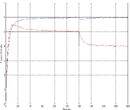
Equations (23) and (24) were used to obtain the process predictions, and the proposed SPC2 technique was then designed using P = [10, 10] and = [0.1, 0.5]. Note that smaller values of p could have been employed without undue alteration of the results that follow. Although the process is highly interacting, to provide a comparative benchmark a baseline level of control can be
achieved using continuous PI controllers. Analysis of the process relative gain array indicates that best results will be achieved
by closing the control loops as {u1, y2} and {u2, y1} [19]. The direct synthesis (or ‘lambda-tuning’) method was then employed for each PI loop individually, with a target time constant of = 5s [20]. In the simulations, which each lasted 200 seconds, an
initial step change in setpoints to r1 = 6 and r2 = 5 was issued. After 120 seconds, r2 was decreased to 4. In each case, a zero-mean band-limited white noise sequence with variance 0.005 and sampling time 0.05 seconds was injected into each
process output; the same random number seeds were employed across both experiments. In order to measure the quality of the
resulting control, the Integral of Squared Error (ISE) between the process outputs and the desired reference trajectory (with
time constant 5 seconds) was also measured in each case. Figs. 5 and 6 show the results obtained for the dual PI and SPC2 controllers, respectively. In the figures, the blue line shows the response of effluent concentration y1 and red line that of the reactor temperature y2.
Fig. 6 Simulation results for SPC2 controller with = [0.1, 0.5].
From the figures obtained, it can be seen that the PI controllers take some time to settle to their corresponding setpoints
(approximately 100 seconds in both cases), with undershoot in r1 and overshoot in r2. Following the change in r2 after 120 seconds, the loop interaction is evident with a disturbance in r1. Settling times in this case are of the order 60 seconds. The ISE
measured for this case was 25.73. For the SPC2 controller, it can be observed that the process variables make a smooth transition to their setpoints, and minimal loop interaction is evident, even following the change in r2 after 120 seconds. Settling times are of the order 20 seconds in all cases. The ISE measured for this case was 5.83, giving a measure of the improved
performance over the dual PI approach. In order to illustrate that in the SPC2 approach, the link between the choice of P values and system robustness is weakened, a further experiment was carried out. The experiment was repeated again using P = [10, 10]
but with increased to [0.4, 2.0]. The simulation result is shown in Fig. 7, where again the blue line shows the response of
effluent concentration y1 and red line that of the reactor temperature y2. A comparison between Fig. 6 and Fig. 7 clearly shows that as expected, the robustness and hence speed of response in the control loop may be altered by appropriate adjustment of ,
without the need to modify the P points. This is reflected in the increased ISE in this case, which was 31.19. However, comparison of the behaviors shown in Figs. 5 and 7, even the detuned SPC2 approach seems preferable to the dual PI as the setpoints are reached more quickly, despite the overshoot; setting times of around 60 seconds are observed. Finally, note that in
the original SPC approach, P would need to be set to ≥ 60 to achieve a similar response to that shown in Fig. 6. This increase
has a marked effect on the quality of the predictions, and a corresponding increase in the ISA value.
5.3. Simulation Results: Constrained Control
As a second validation study, rate constraints of +/- 1.0 unit per 0.5 second were assumed to be present on the process
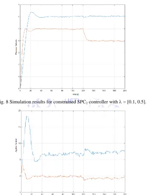
manipulated variables u1 and u2. The proposed SPC2 technique was then applied using the previous configuration of P = [10, 10] and = [0.1, 0.5]. Constraints were handled using the coordinate descent method described in the previous Section, with an epsilon of 10-4 employed. Figs. 8 and 9 display the obtained responses and the applied manipulated variables respectively. As may be seen in Fig.8 the response is actually very close to that of Fig. 7 (detuning of the controller), with an associated increase
in ISE which was recorded as 35.88. Not more than 4 simple inner loop iterations were required to handle the constraints at
each sample (in most cases when the constraints were violated, the saturated solution was quickly detected as optimal in 1
iteration). This gives an illustration that for the relatively small dimensions typical of many industrial multivariable control
loops, the proposed optimization technique is computationally feasible as well as being trivial to implement.
Fig. 8 Simulation results for constrained SPC2 controller with = [0.1, 0.5].
Fig. 9 Applied controls for the constrained SPC2 controller simulation.
6.
Conclusion
It has been argued in this paper that whilst the linear-programming approach to simplified multivariable MPC has many
attractive features, it also has several drawbacks. The paper has then gone on to present the 2-norm approach to simplified
multivariable MPC, and shown that it retains many of the beneficial features of the original whilst overcoming some of these
drawbacks. Preliminary results have been described which provide evidence of the suitability of the proposed technique, and in
conclusion it seems to be a useful adjunct to its linear counterpart. Future work will concentrate upon a more thorough
References
[1]E.F. Camacho and C. Bordons, Model Predictive Control: 2nd Edition. Springer-Verlag London, 2004.
[2]M. Morari and J. H. Lee, “Model predictive control: past, present and future,” Computers and Chemical Engineering, vol. 23, no. 4/5, pp. 667-682, 1999.
[3]D.R. Saffer II and F.J. Doyle III, “Analysis of linear programming in model predictive control,” Computers and Chemical Engineering, vol. 28, pp. 2749-2763, 2004.
[4]Y.P. Gupta, “A simplified predictive control approach for handling constraints through linear programming,” Computers in Industry, vol. 21, no. 3, pp. 255-265, 1993.
[5]R.A. Abou-Jeyab, Y.P. Gupta, J.R. Gervais, P.A. Branchi and S.S. Woo, “Constrained multivariable control of a distillation column using a simplified model predictive control algorithm,” Journal of Process Control, vol. 11, pp. 509-517.
[6]F. Zhao and Y.P. Gupta, “A simplified predictive control algorithm for disturbance rejection,” ISA Transactions, vol. 44, pp. 187-198, 2005.
[7]M. Abu-Ayyad and R. Dubay, “Real-time comparison of a number of predictive controllers,” ISA Transactions, vol. 46, pp. 411-418, 2007.
[8]G.C. Kember, R. Dubay and S.E. Mansour, “On simplified predictive control as a generalization of least-squares dynamic matrix control,” ISA Transactions, vol. 44, 345-352.
[9]Y.P. Gupta, “Solution of low-dimensional constrained model predictive control problems,” ISA Transactions, vol. 43, pp. 499-508.
[10]G.C. Buttazzo, Hard Real-Time Computing Systems: Predictable Scheduling Algorithms and Applications, Spinger-Verlag, New York, 2005.
[11]C.H. Papadimitriou and K. Stieglitz, Combinatorial Optimization: Algorithms and Complexity, Dover Publications Inc., England, 2000.
[12]A. Bjorck, Numerical Methods for Least Squares Problems, SIAM Publishing, Philadelphia, USA, 1996.
[13]G.H. Golub and C.F. Van Loan, Matrix Computations: 3rd edition, Baltimore: Johns Hopkins University Press, 1996. [14]W.H. Press, S.A. Teukolsky, W.T. Vetterling and B.P. Flannery, Numerical Recipes in C: The Art of Scientific
Computing, Cambridge University Press, 1992.
[15]J. Sherman and W. Morrison, “Adjustment of an inverse matrix corresponding to a change in one element of a given matrix,” Annals of Mathematical Statistics, vol. 21, no. 1, pp. 124-127, 1950.
[16]K.J. Astrom and B. Wittenmark, Adaptive Control: 2nd Edition, Addison Wesley, 1995.
[17]B. Schofield, “On Active Set Algorithms for Solving Bound-Constrained Least Squares Control Allocation Problems,” In: Proceedings of the 2008 American Control Conference, Seattle, Washington, USA, June 2008.
[18]Z. Luo and P. Tseng, “On the linear convergence of descent methods for convex essentially smooth minimization,” SIAM Journal of Control and Optimization, vol. 19, no. 3, pp. 368–400, 1992.
[19]M. Bierlaire, Ph.L. Toint and D. Tuyttens, “On iterative algorithms for linear least squares problems with bound constraints,” Linear Algebra and its Applications, vol. 143, pp. 111–143, 1991.
[20]B. Roefel and B.H. Betlem, Advanced practical process control, Springer-Verlag, Berlin, 2004.
![Fig. 7 Simulation results for SPC2 controller with = [0.4, 2].](https://thumb-us.123doks.com/thumbv2/123dok_us/9828500.1968946/12.595.182.419.49.251/fig-simulation-results-spc-controller.webp)