On-Line Sequential Bin Packing
Andr´as Gy¨orgy [email protected]
Machine Learning Research Group
Computer and Automation Research Institute of the Hungarian Academy of Sciences Kende u. 13–17, 1111 Budapest, Hungary
G´abor Lugosi [email protected]
ICREA and Department of Economics Universitat Pompeu Fabra
Ramon Trias Fargas 25–27 08005 Barcelona, Spain
Gy¨orgy Ottucs´ak [email protected]
Department of Computer Science and Information Theory Budapest University of Technology and Economics Magyar Tud´osok K¨or´utja 2
1117 Budapest, Hungary
Editor: Shie Mannor
Abstract
We consider a sequential version of the classical bin packing problem in which items are received one by one. Before the size of the next item is revealed, the decision maker needs to decide whether the next item is packed in the currently open bin or the bin is closed and a new bin is opened. If the new item does not fit, it is lost. If a bin is closed, the remaining free space in the bin accounts for a loss. The goal of the decision maker is to minimize the loss accumulated over n periods. We present an algorithm that has a cumulative loss not much larger than any strategy in a finite class of reference strategies for any sequence of items. Special attention is payed to reference strategies that use a fixed threshold at each step to decide whether a new bin is opened. Some positive and negative results are presented for this case.
Keywords: bin packing, on-line learning, prediction with expert advice
1. Introduction
In the classical off-line bin packing problem, an algorithm receives items (also called pieces) of size
x1,x2, . . . ,xn∈(0,1]. We have an infinite number of bins, each with capacity 1, and every item is to be assigned to a bin. Further, the sum of the sizes of the items (also denoted by xt) assigned to any bin cannot exceed its capacity. A bin is empty if no item is assigned to it, otherwise, it is used. The goal of the algorithm is to minimize the number of used bins. This is one of the classical NP-hard problems and heuristic and approximation algorithms have been investigated thoroughly, see, for example, Coffman et al. (1997).
immediately, without any knowledge of the next pieces. In this setting the goal is the same as in the off-line problem, that is, the number of used bins is to be minimized, see, for example, Seiden (2002).
In both the off-line and on-line problems the algorithm has access to the bins in arbitrary or-der. In this paper we abandon this assumption and introduce a more restricted version that we call
sequential bin packing. In this setting items arrive one by one (just like in the on-line problem)
but in each round the algorithm has only two possible choices: assign the given item to the (only) open bin or to the “next” empty bin (in this case this will be the new open bin), and items cannot be assigned anymore to closed bins. An algorithm thus determines a sequence of binary decisions
i1, . . . ,inwhere it =0 means that the next item is assigned to the open bin and it=1 means that a new bin is opened and the next item is assigned to that bin. Of course, if it=0, then it may happen that the item xtdoes not fit in the open bin. In that case the item is “lost.” If the decision is it=1 then the remaining empty space in the last closed bin is counted as a loss. The measure of performance we use is the total sum of all lost items and wasted empty space.
Just as in the original bin packing problem, we may distinguish off-line and on-line versions of the sequential bin packing problem. In the off-line sequential bin packing problem the entire sequence x1, . . . ,xn is known to the algorithm at the outset. Note that unlike in the classical bin packing problem, the order of the items is relevant. This problem turns out to be computationally significantly easier than its non-sequential counterpart. In Section 3 we present a simple algorithm with running time of O(n2) that minimizes the total loss in the off-line sequential bin packing problem.
Much more interesting is the on-line variant of the sequential bin packing problem. Here the items xt are revealed one by one, after the corresponding decision it has been made. In other words, each decision has to be made without any knowledge on the size of the item. Formulated this way, the problem is reminiscent of an on-line prediction problem, see Cesa-Bianchi and Lugosi (2006). However, unlike in standard formulations of on-line prediction, here the loss the predictor suffers depends not only on the outcome xt and decision it but also on the “state” defined by the fullness of the open bin.
Our goal is to extend the usual bin packing problems to situations in which one can handle only one bin at a time, and items must be processed immediately so they cannot wait for bin changes. To motivate the on-line sequential model, one may imagine a simple revenue management problem in which a decision maker has a unit storage capacity at his disposal. A certain product arrives in packages of different size and after each arrival, it has to be decided whether the stored packages are shipped or not. (Storage of the product is costly.) If the stored goods are shipped, the entire storage capacity becomes available again. If they are not shipped one waits for the arrival of the next package. However, if the next package is too large to fit in the remaining open space, it is lost (it will be stored in another warehouse).
In another example of application, a sensor collects measurements that can be compressed to variable size (these are the items). The sensor communicates its measurements by sending frames of some fixed size (bins). Since it has limited memory, it cannot store more data than one frame. To save energy, the sensor must maximize its throughput (the proportion of useful data in each frame) and at the same time minimize data loss (this trade-off is reflected in the definition of the loss function).
randomized algorithm for the sequential on-line bin packing problem that achieves a cumulative loss (measured as the sum of the total wasted capacity and lost items) that is less than the total loss of the best strategy in the class (determined in hindsight) plus a quantity of the order of n2/3ln1/3N.
Arguably the most natural comparison class contains all algorithms that use a fixed threshold to decide whether a new bin is opened. In other words, reference predictors are parameterized by a real number p∈(0,1]. An expert with parameter p simply decides to open a new bin whenever the remaining free space in the open bin is less than p. We call such an expert a constant-threshold strategy. First we point out that obtaining uniform regret bounds for this class is difficult. We present some impossibility results in relation to this problem. We also offer some data-dependent bounds for an algorithm designed to compete with the best of all constant-threshold strategies, and show that if item sizes are jittered with a certain noise then a uniform regret bound of the order of
n2/3ln1/3n may be achieved .
The principal difficulty of the problem lies in the fact that each action of the decision maker takes the problem in a new “state” (determined by the remaining empty space in the open bin) which has an effect on future losses. Moreover, the state of the algorithm is typically different from the state of the experts which makes comparison difficult. In related work, Merhav et al. (2002) considered a similar setup in which the loss function has a “memory,” that is, the loss of a predictor depends on the loss of past actions. Furthermore, Even-Dar et al. (2005) and Yu et al. (2009) considered theMDP
case where the adversarial reward function changes according to some fixed stochastic dynamics. However, there are several main additional difficulties in the present case. First, unlike in Merhav et al. (2002), but similarly to Even-Dar et al. (2005) and Yu et al. (2009), the loss function has an unbounded memory as the state may depend on an arbitrarily long sequence of past predictions. Second, the state space is infinite (the[0,1)interval) and the class of experts we compare to is also infinite, in contrast to both of the above papers. However, the special properties of the bin packing problem make it possible to design a prediction strategy with small regret.
Note that the MDPsetting of Even-Dar et al. (2005) and Yu et al. (2009) would be a too
pes-simistic approach to our problem, as in our case there is a strong connection between the rewards in different states, thus the absolute adversarial reward function results in an overestimated worst case. Also, in the present case, state transitions are deterministically given by the outcome, the previous state, and the action of the decision maker, while in the setup of Even-Dar et al. (2005) and Yu et al. (2009) transitions are stochastic and depend only on the state and the decision of the algorithm, but not on the reward (or on the underlying individual sequence generating the reward).
We also mention here the similar on-line bin packing with rejection problem where the algorithm has an opportunity to reject some items and the loss function is the sum of the number of the used bins and the “costs” of the rejected items, see He and D´osa (2005).1 However, instead of the number of used bins, we use the sum of idle capacities (missed or free spaces) in the used bins to measure the loss.
The following example may help explain the difference between various versions of the prob-lem.
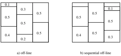
Example 1 Let the sequence of the items beh0.4,0.5,0.2,0.5,0.5,0.3,0.5,0.1i. Then the cumula-tive loss of the optimal off-line bin packing is 0 and it is 0.4 in the case of sequential off-line bin
packing (see Figure 1). In the sequential case the third item (0.2) has been rejected.
0.5 0.5
0.5
0.5
0.5
0.5
0.5 0.5
0.4 0.4
0.3
0.3 0.2
0.1
0.1
a) off-line b) sequential off-line
Figure 1: The difference between the optimal solutions for the off-line and sequential off-line prob-lems.
The rest of the paper is organized as follows. In Section 2 the problem is defined formally. In Section 3 the complexity of the off-line sequential bin packing problem is analyzed. The main results of the paper are presented in Sections 4 and 5.
2. Setup
We use a terminology borrowed from the theory of on-line prediction with expert advice. Thus, we call the sequential decisions of the on-line algorithm predictions and we use forecaster as a synonym for algorithm.
We denote by It ∈ {0,1}the action of the forecaster at time t (i.e., when t−1 items have been received). Action 0 means that the next item will be assigned to the open bin and action 1 represents the fact that a new bin is opened and the next item is assigned to the next empty bin. Note that we assume that we start with an open empty bin, thus for any reasonable algorithm, I1=0, and we
will restrict our attention to such algorithms. The sequence of decisions up to time t is denoted by
It ∈ {0,1}t.
Denote bybst∈[0,1)the free space in the open (last) bin at time t≥1, that is, after having placed the items x1,x2, . . . ,xt according to the sequence It of actions. This is the state of the forecaster. More precisely, the state of the forecaster is defined, recursively, as follows: As at the beginning we have an empty bin,bs0=1. For t=1,2, . . . ,n,
• bst=1−xt, when the algorithm assigns the item to the next empty bin (i.e., It=1);
• bst=bst−1, when the assigned item does not fit in the open bin (i.e., It=0 andsbt−1<xt);
• bst=bst−1−xt, when the assigned item fits in the open bin (i.e., It=0 andbst−1≥xt). This may be written in a more compact form:
b
st = bst(It,xt,sbt−1)
= It(1−xt) + (1−It)(bst−1−I{bst−1≥xt}xt)
whereI{·} denotes the indicator function of the event in brackets, that is, it equals 1 if the event is
true and 0 otherwise. The loss suffered by the forecaster at round t is
where the loss functionℓis defined by
ℓ(0,x|s) =
(
0, if s≥x;
x, otherwise (1)
and
ℓ(1,x|s) =s. (2)
The goal of the forecaster is to minimize its cumulative loss defined by
b
Lt =LIt,t=
t
∑
s=1
ℓ(Is,xs|bss−1).
In the off-line version of the problem, the entire sequence x1, . . . ,xnis given and the solution is the optimal sequence I∗nof actions
I∗n= argmin
In∈{0,1}n
LIn,n.
In the on-line version of the problem the forecaster does not know the size of the next items, and the sequence of items can be completely arbitrary. We allow the forecaster to randomize its decisions, that is, at each time instance t, It is allowed to depend on a random variable Ut where U1, . . . ,Unare i.i.d. uniformly distributed random variables in[0,1].
Since we allow the forecaster to randomize, it is important to clarify that the entire sequence of items are determined before the forecaster starts making decisions, that is, x1, . . . ,xn∈(0,1]are fixed and cannot depend on the randomizing variables. (This is the so-called oblivious adversary model known in the theory of sequential prediction, see, for example, Cesa-Bianchi and Lugosi 2006.)
The performance of a sequential on-line algorithm is measured by its cumulative loss. It is natural to compare it to the cumulative loss of the off-line solution I∗n. However, it is easy to see that in general it is impossible to achieve an on-line performance that is comparable to the optimal solution. (This is in contrast with the non-sequential counterpart of the bin packing problem in which there exist on-line algorithms for which the number of used bins is within a constant factor of that of the optimal solution, see Seiden 2002.)
So in order to measure the performance of a sequential on-line algorithm in a meaningful way, we adopt an approach extensively used in on-line prediction (the so-called “experts” framework). We define a set of reference forecasters, the so-called experts. The performance of the algorithm is evaluated relative to this set of experts, and the goal is to perform asymptotically as well as the best expert from the reference class.
Formally, let fE,t ∈ {0,1}be the decision of an expert E at round t, where E ∈
E
andE
is the set of the experts. This set may be finite or infinite, we consider both cases below. Similarly, we denote the state of expert E with sE,t after the t-th item has been revealed. Then the loss of expert E at round t isℓ(fE,t,xt|sE,t−1)
and the cumulative loss of expert E is
LE,n= n
∑
t=1
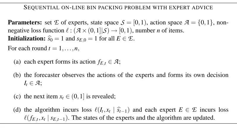
SEQUENTIAL ON-LINE BIN PACKING PROBLEM WITH EXPERT ADVICE
Parameters: set
E
of experts, state spaceS
= [0,1), action spaceA
={0,1}, non-negative loss functionℓ:(A
×(0,1]|S
)→[0,1), number n of items.Initialization: bs0=1 and sE,0=1 for all E∈
E
.For each round t=1, . . . ,n,
(a) each expert forms its action fE,t∈
A
;(b) the forecaster observes the actions of the experts and forms its own decision
It ∈
A
;(c) the next item xt∈(0,1]is revealed;
(d) the algorithm incurs loss ℓ(It,xt |bst−1) and each expert E ∈
E
incurs loss ℓ(fE,t,xt |sE,t−1). The states of the experts and the algorithm are updated.Figure 2: Sequential on-line bin packing problem with expert advice.
The goal of the algorithm is to perform almost as well as the best expert from the reference class
E
(determined in hindsight). Ideally, the normalized difference of the cumulative losses (the so-called
regret) should vanish as n grows, that is, one wishes to achieve
lim sup n→∞
1
n(bLn−Einf∈ELE,n)≤0
with probability one, regardless of the sequence of items. This property is called Hannan
consis-tency, see Hannan (1957). The model of sequential on-line bin packing with expert advice is given
in Figure 2.
In Sections 4 and 5 we design sequential on-line bin packing algorithms. In Section 4 we assume that the class
E
of experts is finite. For this case we establish a uniform regret bound, regardless of the class and the sequence of items. In Section 5 we consider the (infinite) class of experts defined by constant-threshold strategies. This case turns out to be considerably more difficult. We show that algorithms, similar (in some sense) to the one developed for the finite expert classes, cannot work in general in this situation. We provide a data-dependent regret bound for a generalization of the finite-expert algorithm of Section 4, which, in accordance with the previous result, does not guarantee consistency in general. However, we show that if the item sizes are jittered with certain noise, the regret of the algorithm vanishes uniformly regardless of the original sequence of items.But before turning to the on-line problem, we show how the off-line problem can be solved by a simple quadratic-time algorithm.
3. Sequential Off-line Bin Packing
In this section we show that the sequential bin packing problem is significantly easier. Indeed, we offer an algorithm to find the optimal sequential strategy with time complexity O(n2)where n is the number of the items.
The key property is that after the t-th item has been received, the 2t possible sequences of decisions cannot lead to more than t different states.
Lemma 1 For any fixed sequence of items x1,x2, . . . ,xnand for every 1≤t≤n,
|
S
t| ≤t, whereS
t ={s : s=sIt,t,It∈ {0,1}t}
and sIt,t is the state reached after receiving items x1, . . . ,xt with the decision sequence It.
Proof The proof goes by induction. Note that since I1 =0, we always have sI1,1=1−x1, and therefore |
S
1|=1. Now assume that |S
t−1| ≤t−1. At time t, the state of every sequence ofdecisions with It =0 belongs to the set
S
t′={s′: s′=s−I{s≥xt}xt,s∈S
t−1}and the state of thosewith It=1 becomes 1−xt. Therefore,
|
S
t| ≤ |S
t′|+1≤ |S
t−1|+1≤tas desired.
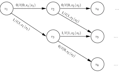
To describe a computationally efficient algorithm to compute I∗n, we set up a graph with the set of possible states as a vertex set (there are O(n2)of them by Lemma 1) and we show that the shortest path on this graph yields the optimal solution of the sequential off-line bin packing problem.
To formalize the problem, consider a finite directed acyclic graph with a set of vertices V = {v1, . . . ,v|V|}and a set of edges E={e1, . . . ,e|E|}. Each vertex vk =v(sk,tk)of the graph is defined by a time index tkand a state sk∈
S
tk and corresponds to state sk reachable after tk steps. To showthe latter dependence, we will write vk∈
S
tk. Two vertices(vi,vj)are connected by an edge if andonly if vi∈
S
t−1, vj∈S
t and state vj is reachable from state vi. That is, by choosing either action 0 or action 1 in state vi, the new state becomes vj after item xt has been placed. Each edge has a label and a weight: the label corresponds to the action (zero or one) and the weight equals the loss, depending on the initial state, the action, and the size of the item. Figure 3 shows the proposed graph. Moreover a sink vertex v|V| is introduced that is connected with all vertices inS
n. These edges have weight equal to the loss of the final states. These losses only depend on the initial state of the edges. More precisely, for(vi,v|V|)the loss is 1−si, where vi∈S
n.Notice that there is a one to one correspondence between paths from v1 to v|V| and possible
sequences of actions of length n. Furthermore, the total weight of each path (calculated as the sum of the weights on the edges of the path) is equal to the loss of the corresponding sequence of actions. Thus, if we find a path with minimal total weight from v1to v|V|, we also find the optimal sequence
of actions for the off-line bin packing problem. It is well known that this can be done in O(|V|+|E|) time.2
Now by Lemma 1, |V| ≤n(n+1)/2+1, where the additional vertex accounts for the sink. Moreover it is easy to see that|E| ≤n(n−1) +n=n2. Hence the total time complexity of finding the off-line solution is O(n2).
v1 v2
v3
v4
v5
v6 . . .
. . . . . .
0/ℓ(0,x1|s1)
1/ℓ (1,
x1 |s1)
0/ℓ(0,x2|s2)
1/ℓ(1,x2|s3)
0/ℓ (0,x2
|s3) 1/ℓ
(1,x 2|s2)
Figure 3: The graph corresponding to the off-line sequential bin packing problem.
4. Sequential On-line Bin Packing
In this section we study the sequential on-line bin packing problem with expert advice, as described in Section 2. We deal with two special cases. First we consider finite classes of experts (i.e., reference algorithms) without any assumption on the form or structure of the experts. We construct a randomized algorithm that, with large probability, achieves a cumulative loss not larger than that of the best expert plus O(n2/3ln1/3N)where N=|
E
|is the number of experts.The following simple lemma is a key ingredient of the results of this section. It shows that in sequential on-line bin packing the cumulative loss is not sensitive to the initial states in the sense that the cumulative loss depends on the initial state in a minor way.
Lemma 2 Let i1, . . . ,im∈ {0,1}be a fixed sequence of decisions and let x1, . . . ,xm∈(0,1] be a sequence of items. Let s0,s′0∈[0,1)be two different initial states. Finally, let s0, . . . ,smand s′0, . . . ,s′m denote the sequences of states generated by i1, . . . ,imand x1, . . . ,xm starting from initial states s0 and s′0, respectively. Then
m
∑
t=1ℓ(it,xt |s′t−1)− m
∑
t=1
ℓ(it,xt |st−1)
≤s ′
0+s0≤2.
Proof Let m′ denote the smallest index for which im′ =1. Note that st−1=st′−1 for all t >m′.
Therefore, we have
m
∑
t=1
ℓ(it,xt |s′t−1)− m
∑
t=1
ℓ(it,xt |st−1)
=
m′
∑
t=1
ℓ(it,xt|s′t−1)− m′
∑
t=1
ℓ(it,xt|st−1)
=
m′−1
∑
t=1
ℓ(0,xt|s′t−1)− m′−1
∑
t=1
Now using the definition of the loss (see Equations 1 and 2), we write
m
∑
t=1
ℓ(it,xt |s′t−1)− m
∑
t=1
ℓ(it,xt |st−1)
=
m′−1
∑
t=1
xt(I{st′−1<xt}−I{st−1<xt}) +s
′
m′−1−sm′−1
≤
m′−1
∑
t=1
xt(1−I{st−1<xt}) +s
′
m′−1−sm′−1
≤
m′−1
∑
t=1
xt(1−I{st−1<xt}) +s′0
≤ s0+s′0
where the next-to-last inequality holds because s′m′−1 ≤s′0 and sm′−1 ≥0, and the last inequality
follows from the fact that
0≤sm′−1 = sm′−2−I{s
m′−2≥xm′−1}xm′−1
= sm′−3−I{s
m′−3≥xm′−2}xm′−2−I{sm′−2≥xm′−1}xm′−1
= s0− m′−1
∑
t=1 I
{st−1≥xt}xt .
Similarly,
m
∑
t=1
ℓ(it,xt |st−1)− m
∑
t=1
ℓ(it,xt |st′−1)≤s′0+s0
and the statement follows.
The following example shows that the upper bound of the lemma is tight.
Example 2 Let x1=s0, s′0<s0, and m′=2. Then m
∑
t=1
ℓ(it,xt |s′t−1)− m
∑
t=1
ℓ(it,xt |st−1)
= ℓ(0,x1|s0′) +ℓ(1,x2|s′1)− ℓ(0,x1|s0) +ℓ(1,x2|s1)
= ℓ(0,s0|s′0) +ℓ(1,x2|s0′)− ℓ(0,s0|s0) +ℓ(1,x2|0) = s0+s′0−(0+0).
Now we consider the on-line sequential bin packing problem when the goal of the algorithm is to keep its cumulative loss close to the best in a finite set of experts. In other words, we assume that the class of experts is finite, say|
E
|=N, but we do not assume any additional structure of theexperts. The ideas presented here will be used in Section 5 when we consider the infinite class of constant-threshold experts.
segments of length m, and, if m does not divide n, an extra segment of length less than m. At the beginning of each segment, the algorithm selects an expert randomly, according to an exponentially weighted average distribution. During the entire segment, the algorithm follows the advice of the selected expert. By changing actions so rarely, the algorithm achieves a certain synchronization with the chosen expert, since the effect of the difference in the initial states is minor, according to Lemma 2. (A similar idea was used in Merhav et al. (2002) in a different context.) The algorithm is described in Figure 4. Recall that each expert E∈
E
recommends an action fE,t∈ {0,1}at every time instance t=1, . . . ,n. Since we have N experts, we may identifyE
with the set{1, . . . ,N}. Thus, experts will be indexed by the positive integers i∈ {1, . . . ,N}. At the beginning of each segment, the algorithm chooses expert i randomly, with probability pi,t, where the distribution pt= (p1,t, . . . ,pN,t) is specified in the algorithm. The random selection is made independently for each segment.The following theorem establishes a performance bound of the algorithm. Recall thatbLndenotes the cumulative loss of the algorithm while Li,nis that of expert i.
Theorem 3 Let n, N≥1, η>0, 1≤m≤n, and δ∈(0,1). For any sequence x1, . . . ,xn∈(0,1] of items, the cumulative loss bLn of the randomized strategy defined in Figure 4 satisfies for all i=1, . . . ,N, with probability at least 1−δ,
b
Ln≤Li,n+ m
ηln
1
wi,0
+nη 8 + r nm 2 ln 1 δ+ 2n
m +2m.
In particular, choosing wi,0=1/N for all i=1, . . . ,N, m= (16n/ln(N/δ))1/3andη=
p
8m ln N/n, one has
b
Ln− min
i=1,...,NLi,n≤ 3 3
√ 2n
2/3ln1/3N
δ +4
2n ln(N/δ)
1/3
.
Proof We introduce an auxiliary quantity, the so-called hypothetical loss, defined as the loss the
algorithm would suffer if it had been in the same state as the selected expert. This hypothetical loss does not depend on previous decisions of the algorithm. More precisely, the true loss of the algorithm at time instance t isℓ(It,xt |bst)and its hypothetic loss isℓ(It,xt |sJt,t). Introducing the
notation
ℓi,t=ℓ(fi,t,xt|si,t), the hypothetical loss of the algorithm is just
ℓ(It,xt|sJt,t) =ℓ(fJt,t,xt |sJt,t) =ℓJt,t .
Now it follows by a well-known result of randomized on-line prediction (see, e.g., Lemma 5.1 and Corollary 4.2 in Cesa-Bianchi and Lugosi, 2006) that the hypothetical loss of the sequential on-line bin packing algorithm satisfies simultaneously for all i=1, . . . ,N, with probability at least 1−δ,
n
∑
t=1 ℓJt,t ≤
n
∑
t=1 ℓi,t+m
1
ηln
1
wi,0
+n′η
8 + r n′ 2 ln 1 δ !
+m, (3)
where n′=⌊n
m⌋and the last m term comes from bounding the difference on the last, not necessarily complete segment. Now we may decompose the regret relative to expert i as follows:
b
Ln−Li,n= bLn− n
∑
t=1 ℓJt,t
!
+
n
∑
t=1
ℓJt,t−Li,n !
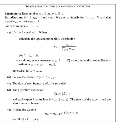
SEQUENTIAL ON-LINE BIN PACKING ALGORITHM
Parameters: Real numberη>0 and m∈N+.
Initialization: bs0=1, si,0=1 and wi,0>0 are set arbitrarily for i=1, . . . ,N such that w1,0+w2,0+···+wN,0=1.
For each round t=1, . . . ,n,
(a) If((t−1)mod m) =0 then
– calculate the updated probability distribution
pi,t=
wi,t−1
∑N
j=1wj,t−1
for i=1, . . . ,N;
– randomly select an expert Jt∈ {1, . . . ,N}according to the probability dis-tribution pt = (p1,t, . . . ,pN,t);
otherwise, let Jt =Jt−1.
(b) Follow the chosen expert: It= fJt,t.
(c) The size of next item xt ∈(0,1]is revealed.
(d) The algorithm incurs loss
ℓ(It,xt|bst−1)
and each expert i incurs lossℓ(fi,t,xt|si,t−1). The states of the experts and the
algorithm are changed.
(e) Update the weights
wi,t =wi,t−1e−ηℓ(fi,t,xt|si,t−1)
for all i∈ {1, . . . ,N}.
Figure 4: Sequential on-line bin packing algorithm.
The second term on the right-hand side is bounded using (3). To bound the first term, observe that by Lemma 2,
b
Ln− n
∑
t=1
ℓJt,t =
n
∑
t=1
ℓ(It,xt|bst−1)− n
∑
t=1
ℓ(It,xt |sJt−1,t−1)
≤ m+
n′−1
∑
s=0 m
∑
t=1
ℓ(Ism+t,xsm+t|bssm+t−1)−ℓ(Ism+t,xsm+t|sJsm+t−1,sm+t−1)
≤ m+2n′
5. Constant-threshold Experts
In this section we address the sequential on-line bin packing problem when the goal is to perform almost as well as the best in the class of all threshold strategies. Recall that a constant-threshold strategy is parameterized by a number p∈(0,1]and it opens a new bin if and only if the remaining empty space in the bin is less than p. More precisely, if the state of the algorithm defined by expert with parameter p is sp,t−1, then at time t the expert’s advice is I{sp,t−1<p}. To simplify notation, we will refer to each expert with its parameter, and, similarly to the previous section, fp,t and sp,t will denote the decision of expert p at time t, and its state after the decision, respectively.
The difficulty in this setup is that there are uncountably many constant-threshold experts. The simplest possibility is to discretize the class. For example, by considering the set of constant-threshold experts with values of p in the set{1/N,2/N, . . . ,1}and using the randomized algorithm described in the previous section, we immediately obtain that the cumulative regret of the algorithm, when compared to the best constant-threshold expert with p in this set is bounded by O(n2/3ln1/3N) with high probability. It is natural to suspect that if N is large, the loss of the best discretized constant-threshold expert is not much larger than that corresponding to the best (unrestricted) value of p∈(0,1]. However, this is not true in general. The next lemma shows that any such discretization is doomed to failure, at least in the worst-case sense. We denote by Lp,nthe cumulative loss of the constant-threshold expert indexed by p∈(0,1].
Lemma 4 For all n such that n/4 is a positive integer and 1/2<a<b≤1 there exists a sequence
x1, . . . ,xnof items such that
sup p∈(a,b]
Lp,n< inf
p∈/(a,b]Lp,n− n
4+3
for any values of the initial states sp,0∈[p,1],p∈(0,1].3
Proof Given 1/2≤a<b≤1, we construct a sequence with the announced property. The first fourth of the sequence is defined by x1=1−a and x2=···=xn/4=1. If an expert asks for a new
bin after the first item then it suffers no loss for t=2, . . . ,n/4, thus the cumulative loss up to time
n/4 is bounded as Lp,n/4≤1. Note that any expert with parameter p>a is such, as the first item
always fits the actual bin, as by the conditions of the lemma 1−a≤a<p≤sp,0, but then the empty
space becomes s0,p−(1−a)≤a<p, and so expert p opens a new bin. In case of an expert with parameter q≤a, it depends on the initial state if the expert opens a new bin. If the actual bin is left
open after the first item then the expert suffers loss Lq,n/4=n/4−1. In particular, if sq,0=1 then
after the first item expert q moves to state sq,1=a and leaves the bin open. Thus, after time n/4 an
expert either suffers loss at least n/4−1 (then the parameter of the expert is at most a), or it suffers loss at most 1, but then it is in the state sp,n/4=1. Now for the second forth of the sequence repeat
the first one, that is, let xn/4+1=1−a, xn/4+2=···=xn/2=1. By the above argument we can see
that if an expert with parameter q≤a does not suffer large loss up to time n/4 then it starts with an empty bin and suffers a large loss in the second fourth of the segment. Thus, Lq,n/2≥n/4−1 for
any q≤a. On the other hand, for any expert p>a we have Lp,n/2<2 and sp,n/2=1.
3. Note that for any expert p∈(0,1], sp,t∈[p,1]for all t≥1 regardless of the initial state, and so it is natural to restrict
After this point of time, let xn/2+1=1−b, xn/2+2=b and repeat this pair of items n/4 times.
After receiving xn/2+1=1−b, every expert with parameter p∈(a,b]keeps the bin open and
there-fore does not suffer any loss after receiving the next item. On the other hand, experts with parameter
r>b close the bin, suffer loss b, and after xn/2+2=b is received, once again they close the bin and
suffer loss 1−b (here we used the fact that r>1−b since we assumed b>1/2. Thus, between periods n/2+1 and n, all experts with p∈(a,b]suffer zero loss while experts with parameter r>b
suffer loss n/4.
Summarizing, for the sequence
1−a, 1,1, . . . ,1
| {z }
n/4−1 periods
,1−a, 1,1, . . . ,1
| {z }
n/4−1 periods
,1−b,b,1−b,b. . . ,1−b,b
| {z }
n/2 periods
,
we have
Lp,n
<2 if p∈(a,b]
≥n/4−1 if p≤a
≥n/4 if p>b.
Lemma 4 implies that one cannot expect a small regret with respect to all possible constant-threshold experts. This is true for any algorithm that, as the one proposed in the previous section, divides time into segments and on each segment chooses a constant-threshold expert and acts as the chosen expert during the following segment. Recall that this segmentation was necessary to make sure that the state of the algorithm gets synchronized with the chosen one. The statement is formalized below.
Theorem 5 Consider any sequential on-line bin packing algorithm that divides time into segments of lengths m1,m2, . . . ,mk≥3 (where∑ki=1mi=n) such that, at the beginning of each segment mi, the algorithm chooses (in a possibly randomized way) a parameter pi∈(0,1]and follows this expert during the segment, that is, It =I{bst−1<pi} for all t =∑
i−1
j=1mj+1, . . . ,∑ij=1mj. Then there exists a sequence of items x1, . . . ,xn such that the loss of the algorithm satisfies, with probability at least 1/2,
b
Ln≥ inf
p∈(0,1]Lp,n+ n
4−6k.
Proof We construct the sequence of items using the sequence shown in the proof of Lemma 4 as a
building block. At time 1, divide the interval(0,1]into 2k subintervals of equal length and choose one of these intervals uniformly at random. Denote the end points of this interval by(A1,B1]. Then during the first segment we define the items by
1−A1, 1,1, . . . ,1
| {z }
⌊m1/4⌋−1 periods
,1−A1, 1,1, . . . ,1
| {z }
⌊m1/4⌋−1 periods
,1−B1,B1,1−B1,B1. . . ,1−B1,B1
| {z }
⌊m1/2⌋periods
.
If m1 is not divisible by 4, we may define the remaining (at most three) items arbitrarily. Then,
the possibility that m1 is not divisible by 4.) However, no matter how the algorithm chooses the
expert to follow, the probability that it finds the correct subinterval is 1/(2k).
To continue the construction, we now divide the interval(A1,B1]into 2k intervals of equal length and choose one at random, say(A2,B2]. We define the next items similarly to the first segment, but now we make sure that the optimal constant-threshold expert falls in the interval(A2,B2], that is,
the items of the second segment are defined by
1−A2, 1,1, . . . ,1
| {z }
⌊m2/4⌋−1 periods
,1−A2, 1,1, . . . ,1
| {z }
⌊m2/4⌋−1 periods
,1−B2,B2,1−B2,B2. . . ,1−B2,B2
| {z }
⌊m2/2⌋periods
.
As before, if m2is not divisible by 4, we may define the remaining (at most three) items arbitrarily.
Once again, the excess loss of the algorithm, when compared to the best constant-threshold expert, is at least m24 −6 with probability 1/(2k).
We may continue the same randomized construction of the item sizes in the same manner, always dividing the previously chosen interval into 2k equal pieces, choosing one at random, and constructing the item sequence so that experts in the chosen interval are significantly better than any other expert.
By the union bound, the probability that the forecaster never chooses the correct interval is at least 1/2, so with probability at least 1/2,
b
Ln− inf
p∈(0,1]Lp,n≥ k
∑
i=1
mi
4 −6
=n 4−6k
as desired.
The theorem above shows that if one uses a segmentation for synchronization purposes, one cannot expect nontrivial regret bounds that hold uniformly over all possible sequences of items and for all constant-threshold experts, unless the number of segments is proportional to n. It seems unlikely that without such synchronization one may achieve o(n)regret. Unfortunately, we do not have a formal proof for arbitrary algorithms (that do not divide time into segments).
However, one may still obtain meaningful regret bounds that depend on the data. We derive such a bound next. We also show that under some natural restrictions on the item sizes, this result allows us to derive regret bounds that hold uniformly over all constant-threshold experts.
In order to understand the structure of the problem of constant-threshold experts, it is important to observe that on any sequence of n items, experts can exhibit only a finite number of different be-haviors. In a sense, the “effective” number of experts is not too large and this fact may be exploited by an algorithm.
For t=1, . . . ,n we call two experts t-indistinguishable (with respect to the sequence of items x1, . . . ,xt−1) if their decision sequences are identical up to time t (note that any two experts are
1-indistinguishable, as all experts p start with a decision fp,1=0). This property defines a
nat-ural partitioning of the class of experts into maximal t-indistinguishable sets, where any two ex-perts that belong to the same set are t-indistinguishable, and exex-perts from different sets are not
The first step in proving this fact is the next lemma that shows that the maximal t-indistinguishable expert sets are intervals.
Lemma 6 Let 1≥ p>r >0 be such that expert p and expert r are t-indistinguishable. Then
for any p>q>r expert q is t-indistinguishable from both experts p and r. Thus, the maximal t-indistinguishable expert sets form subintervals of(0,1].
Proof By the assumption of the lemma the decision sequences of experts p and r coincide, that is,
fp,u= fr,u and sp,u=sr,u
for all u=1,2, . . . ,t. Let t1,t2, . . .denote the time instances when expert p (or expert r) assigns the
next item to the next empty bin (i.e., fp,u=1 for u=t1,t2, . . .). If expert q also decides 1 at time tk for some k, then it will decide 0 for t=tk+1, . . . ,tk+1−1 since so does expert p and p>q, and will
decide 1 at time tk+1as q>r. Thus the decision sequence of expert q coincides with that of expert p and r for time instances tk+1, . . . ,tk+1 in this case. Since all experts start with the empty bin at
time 0, the statement of the lemma follows by induction.
Based on the lemma we can identify the t-indistinguishable sets by their end points. Let
Q
t ={q1,t, . . . ,qNt,t} denote the set of the end points after receiving t−1 items, where Nt =|
Q
t|is the number of maximal t-indistinguishable sets, and q0,t=0<q1,t <q2,t<···<qNt,t =1. Then thet-indistinguishable sets are(qk−1,t,qk,t]for k=1, . . . ,Nt. The next result shows that the number of maximal t-indistinguishable sets cannot grow too fast.
Lemma 7 The number of the maximal t-indistinguishable sets is at most quadratic in the number of the items t. More precisely, Nt≤1+t(t−1)/2 for any 1≤t≤n.
Proof The proof is by induction. First, N1=1 (and
Q
1 ={1}) since the first decision of eachexpert is 1. Now assume that Nt ≤1+t(t−1)/2 for some 1≤t≤n−1. When the next item xt arrives, an expert p with state s decides 1 in the next step if and only if 0≤s−xt <p. There-fore, as each expert belonging to the same indistinguishable set has the same state, the k-th max-imal (t−1)-indistinguishable interval with state s is split into two subintervals if and only if
qk−1,t−1<s−xt ≤qk,t−1 (experts in this interval with parameters larger than s−xt will form one subset, and the ones with parameter at most s−xt will form the other one). As the number of possible states after t decisions (the number of different possible values of s−xt) is at most t by Lemma 1, it follows that at most t intervals can be split, and so Nt+1≤Nt+t≤1+t(t+1)/2, where the second inequality holds by the induction hypothesis.
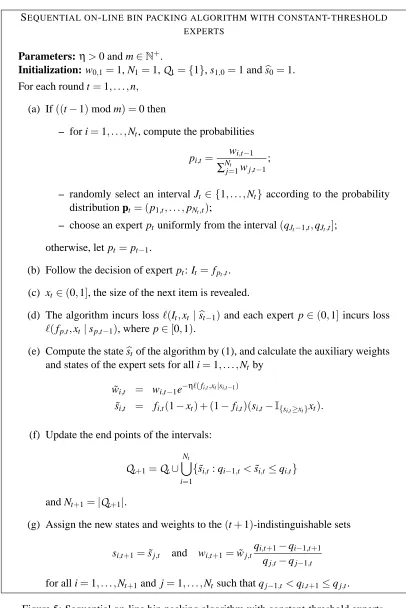
SEQUENTIAL ON-LINE BIN PACKING ALGORITHM WITH CONSTANT-THRESHOLD EXPERTS
Parameters: η>0 and m∈N+.
Initialization: w0,1=1, N1=1,
Q
1={1}, s1,0=1 andbs0=1.For each round t=1, . . . ,n,
(a) If((t−1)mod m) =0 then
– for i=1, . . . ,Nt, compute the probabilities
pi,t=
wi,t−1
∑Nt
j=1wj,t−1
;
– randomly select an interval Jt ∈ {1, . . . ,Nt}according to the probability distribution pt = (p1,t, . . . ,pNt,t);
– choose an expert pt uniformly from the interval(qJt−1,t,qJt,t];
otherwise, let pt=pt−1.
(b) Follow the decision of expert pt: It= fpt,t. (c) xt ∈(0,1], the size of the next item is revealed.
(d) The algorithm incurs lossℓ(It,xt |bst−1) and each expert p∈(0,1]incurs loss ℓ(fp,t,xt|sp,t−1), where p∈[0,1).
(e) Compute the statesbt of the algorithm by (1), and calculate the auxiliary weights and states of the expert sets for all i=1, . . . ,Nt by
˜
wi,t = wi,t−1e−ηℓ(fi,t,xt|si,t−1)
˜
si,t = fi,t(1−xt) + (1−fi,t)(si,t−I{si,t≥xt}xt).
(f) Update the end points of the intervals:
Q
t+1=Q
t∪ Nt[
i=1
{s˜i,t: qi−1,t <s˜i,t≤qi,t}
and Nt+1=|
Q
t+1|.(g) Assign the new states and weights to the(t+1)-indistinguishable sets
si,t+1=s˜j,t and wi,t+1=w˜j,t
qi,t+1−qi−1,t+1 qj,t−qj−1,t
for all i=1, . . . ,Nt+1and j=1, . . . ,Nt such that qj−1,t<qi,t+1≤qj,t.
Up to step (e) the algorithm is essentially the same as in the case of finitely many experts. The two-level random choice of the expert is performed in step (a). In step (f) we update the t-indistinguishable sets, and usually introduce new t-indistinguishable expert sets. Because of these new expert sets, the update of the weights wi,t and the states si,t are performed in two steps, (e) and (g), where the actual update is made in step (e), and reordering of these quantities according to the new indistinguishable sets is performed in step (g) together with the introduction of the weights and states for the newly formed expert sets. (Note that in step (g) the factor(qi,t+1−qi−1,t+1)/(qj,t− qj−1,t)is the proportion of the lengths of the indistinguishable intervals expert qi,t+1 belongs to at
times t+1 and t.)
The performance and complexity of the algorithm is given in the next theorem.
Theorem 8 Let n≥1, η>0, 1≤m≤n, andδ∈(0,1). For any sequence x1, . . . ,xn∈(0,1]of items, the cumulative lossbLn of the randomized strategy defined above satisfies for all p∈(0,1], with probability at least 1−δ,
b
Ln≤Lp,n+ m
ηln
1
lp,n
+nη 8 +
r
nm
2 ln 1
δ+
2n
m +2m
where lp,nis the length of the maximal n-indistinguishable interval that contains p. Moreover, the algorithm can be implemented with time complexity O(n3)and space complexity O(n2).
Remark 9 (i) By choosing m∼n1/3andη∼n−1/3, the regret bound is of the order of n2/3ln(1/l p,n). Note that the constant ln(1/lp,n)reflects the difficulty of the problem (similarly to, for example, the notion of margin in classification, lp,nmeasures the freedom in choosing an optimal decision bound-ary, that is, an optimal threshold). If the indistinguishable interval containing the optimal experts is small, then the problem is hard (and the corresponding penalty term in the bound is large). On the other hand, as Nn≤1+n(n−1)/2, if the classes of indistinguishable experts are more or less of uniform size, then the corresponding term in the bound is of the order of ln n. We show below that this is always the case if there is a certain randomness in the item sizes.
(ii) The way of splitting the weight between new maximal indistinguishable classes in step (g) could be modified in many different ways. For example, instead of assigning weights proportionally to the length of the new intervals, one could simply give half of the weight to both new classes. In this case, instead of the term ln(1/lp∗,n) for the optimal expert p∗, we would get in the bound the number of splits performed until reaching the optimal maximal n-indistinguishable class. The hardness of the problem comes from the fact that the partitioning of the experts into maximal indis-tinguishable classes is not known in advance. If we knew it, we could just simply apply the algorithm of Theorem 3 to the resulting Nnexperts (as in Theorem 4.1 of Cesa-Bianchi and Lugosi, 2006) to obtain a uniformly good bound over all constant-threshold experts.
Proof It is easy to see that the two-level choice of the expert pt ensures that the algorithm is the same as for the finite expert class with the experts defined by
Q
nwith initial weights wi,0=lqi,n,n=qi,n−qi−1,nfor the n-indistinguishable expert class containing qi,n. Thus, Theorem 3 can be used to bound the regret, where the number of experts is Nt.
round), and has to compute the probabilities once in every m step, which requires O(n3/m) compu-tations. Thus the time complexity of the algorithm is O(n3).
Next we use Theorem 8 to show that, for many natural sequences of items, the algorithm above guarantees a small regret uniformly for all constant-threshold experts. In particular, we show that if item sizes are jittered by random noise, then the algorithm shown above has a small regret with respect to all constant-threshold experts (it is well-known that, for general systems, intro-ducing such random perturbations often reduces the sensitivity, and hence results in a more uni-form peruni-formance, for different values of the input). To this end, we simply need to show that
n-indistinguishable intervals cannot be too short. We consider a simple model when the item sizes
are noisy versions of an arbitrary fixed sequence. For simplicity we assume that the noise is uni-formly distributed but the result remains true under more general circumstances. For illustration purposes the simplified model is sufficient.
Theorem 10 Let y1, . . . ,yn∈(0,1]be arbitrary and define the item sizes by
xt=
yt+σt if yt+σt ∈(0,1] 1 if yt+σt >1 0 if yt+σt ≤0
where σ1, . . . ,σn are independent random variables, uniformly distributed on the interval [−ε,ε] for someε>0. If the algorithm of Figure 5 is used with parameters m= (16n/ln(n5/εδ))1/3and
η=p8m ln(n5/ε)/n, then with probability at least 1−δ−1/(4n), one has
b
Ln− min
p∈(0,1]Lp,n≤
3 3
√ 2n
2/3ln1/3n5
εδ+4
2n ln(n5/εδ)
1/3
. (4)
Proof The result follows directly from Theorem 8 if we show that the length of the shortest maximal n-indistinguishable interval is at mostε/n5with probability at least 1−1/(4n)(with respect to the
distribution of the random noise). A very crude bounding suffices to show this. Simply recall from the proof of Lemma 7 that, at time t, a maximal t-indistinguishable interval(p,q)is split if and only if xt∈(s+p,s+q)where s denotes the state of a corresponding constant-threshold expert. Note that
(s+p,s+q)⊆(0,1), since xt=0 or xt =1 cannot split any maximal t-indistinguishable interval, but any such interval can be split by an appropriately chosen xt. At time t there are at most t2/2 different maximal t-indistinguishable intervals and at most t different states, so by the union bound, the probability that there exists a maximal t-indistinguishable interval of length at mostε/n5that is
split at time t is bounded by t3/2 times the probability that xt∈(s+p,s+q)for a fixed interval with q−p≤ε/n5. Because of the assumption on how x
tis generated, the latter probability is bounded by
(q−p)/(2ε)≤1/(2n5)(the truncation of xt at 0 and 1 has no effect, because(s+p,s+q)⊆(0,1)). Hence, the probability that there exists a maximal t-indistinguishable interval of length at mostε/n5
that is split at time t is no more than t3/2·1/(2n5)≤1/(4n2). Thus, using the union bound again, the probability that during the n rounds of the game there exists any maximal t-indistinguishable interval of length at mostε/n5that is split is at most 1/(4n), and therefore, with probability at least
Remark 11 (i) The theorem above shows that, for example, ifε=Ω(n−a)for some a>0 (i.e., if
the noise level is not too small), then the regret with respect to the best constant-threshold expert is O(n2/3ln1/3n).
(ii) A similar model can be obtained, if, instead of having perturbed item sizes, the experts observe the free space in their bins with some noise. Thus, instead of sp,t−1, expert p observes sp,t−1+σp,t truncated to the interval [0,1], and makes decision fp,t based on this value. As in the case of Theorem 10, we assume that the noise is independent over time, that is, the random ensembles{σp,t}p∈(0,1] are independent for all t. If each component is identical, that is,σp,t =σt for all p∈(0,1], then essentially the same argument applies as in the previous theorem, and so
(4) holds if the sequence σ1, . . . ,σn satisfies the assumptions of Theorem 10. On the other hand, if the components of the vectors are also independent, then the problem becomes more difficult, as the t-indistinguishable classes may not be disjoint intervals anymore. An intermediate assumption on the noise that still guarantees that (4) holds for this scenario is that σp,t =σq,t if p and q are t-indistinguishable. Then the same argument as in Theorem 10 works with the only difference (omitting the effects of truncation to [0,1]) that here we have to estimate the probability that xt ∈
(s+p+σt,q,s+q+σt,q)for a fixed xt instead of estimating the probability that xt ∈(s+p,s+q) with a randomized xt. However, it is easy to see that the same bound holds in both cases.
Finally, we present a simple example that reveals that the loss of the best expert can be arbitrarily far from that of the optimal sequential off-line packing.
Example 3 Let the sequence of items be
hε,1−ε,ε,1−ε, . . . ,ε,1−ε
| {z }
2k
,ε,1,1, . . . ,1
| {z }
k
i,
where the number of items is n=3k+1 and 0<ε<1/2. An optimal sequential off-line packing
is achieved if we drop any of theεterms; then the total loss isε. In contrast to this, the loss of any constant-threshold expert is 1−ε+k independently of the choice of the parameter p. Namely, if p≤1−εthen the loss is 0 for the first 2k items, but after the algorithm is stuck and suffers k+1−ε
loss. If p>1−ε, then the loss is k for the first 2k items and after that 1−ε for the rest of the sequence.
6. Conclusions
In this paper we provide an extension of the classical bin packing problems to an on-line sequential scenario. In this setting items are received one by one, and before the size of the next item is revealed, the decision maker needs to decide whether the next item is packed in the currently open bin or the bin is closed and a new bin is opened. If the new item does not fit, it is lost. If a bin is closed, the remaining free space in the bin accounts for a loss. The goal of the decision maker is to minimize the loss accumulated over n periods.
cumulative loss can be made not much larger than that of any strategy that uses a fixed threshold at each step to decide whether a new bin is opened. An interesting aspect of the problem is that the loss function has an (unbounded) memory. The presented solutions rely on the fact that one can “synchronize” the loss function in the sense that no matter in what state an algorithm is started, its loss may change only by a small additive constant. The result for constant-threshold experts is obtained by a covering of the uncountable set of constant-threshold experts such that the cardinality of the chosen finite set of experts grows only quadratically with the sequence length. The approach in the paper can easily be extended to any control problem where the loss function has such a synchronizable property.
Acknowledgments
The authors would like to thank Robert Kleinberg for pointing out a crucial mistake in the earlier version (Gy¨orgy et al., 2008) of this paper. In that paper we erroneously claimed that it was possible to construct a sequential on-line bin packing algorithm that has a small regret with respect to all constant-threshold experts for all possible item sequences.
The authors acknowledge support by the Hungarian Scientific Research Fund (OTKA F60787), by the Mobile Innovation Center of Hungary, by the Spanish Ministry of Science and Technology grant MTM2009-09063, and by the PASCAL2 Network of Excellence under EC grant no. 216886.
References
J. Boyar, L. Epstein, L. M. Favrholdt, J. S. Kohrt, K. S. Larsen, M. M. Pedersen, and S. Wøhlk. The maximum resource bin packing problem. Theoretical Computer Science, 362:127–139, 2006.
N. Cesa-Bianchi and G. Lugosi. Prediction, Learning, and Games. Cambridge University Press, to appear, Cambridge, 2006.
E. G. Coffman, M. R. Garey, and D. S. Johnson. Approximation algorithms for bin packing: a survey. In Approximation Algorithms for NP-hard Problems, pages 46–93. PWS Publishing Co., Boston, MA, 1997.
E. Even-Dar, S. M. Kakade, and Y. Mansour. Experts in a markov decision process. In L. K. Saul, Y. Weiss, and L. Bottou, editors, Advances in Neural Information Processing Systems 17, pages 401–408, Cambridge, MA, 2005. MIT Press.
A. Gy¨orgy, G. Lugosi, and Gy. Ottucs´ak. On-line sequential bin packing. In Proceedings of the 21st
Annual Conference on Learning Theory, COLT 2008, pages 447–454, Helsinki, Finland, July
2008.
J. Hannan. Approximation to bayes risk in repeated plays. In M. Dresher, A. Tucker, and P. Wolfe, editors, Contributions to the Theory of Games, volume 3, pages 97–139. Princeton University Press, 1957.
Y. He and Gy. D´osa. Bin packing and covering problems with rejection. In Proceedings of the 11th
3595 of Lecture Notes in Computer Science, pages 885–894, Kunming, China, August 2005. Springer Berlin/Heidelberg.
N. Merhav, E. Ordentlich, G. Seroussi, and M. J. Weinberger. On sequential strategies for loss functions with memory. IEEE Transactions on Information Theory, 48:1947–1958, 2002.
S. S. Seiden. On the online bin packing problem. Journal of the ACM, 49(5):640–671, 2002.
J. Y. Yu, S. Mannor, and N. Shimkin. Markov decision processes with arbitrary reward processes.