Ranking Forests

(1)

Ranking Forests

Stéphan Clémençon [email protected]

Marine Depecker [email protected]

Institut Telecom LTCI - UMR Telecom ParisTech/CNRS No. 5141 Telecom ParisTech

46 rue Barrault, Paris, 75634, France

Nicolas Vayatis [email protected]

CMLA - UMR ENS Cachan/CNRS No. 8536 ENS Cachan

61, avenue du Pr´esident Wilson, Cachan, 94230, France

Editor:Tong Zhang

Abstract

The present paper examines how the aggregation and feature randomization principles underlying the algorithm RANDOM FOREST(Breiman, 2001) can be adapted tobipartite ranking. The ap-proach taken here is based on nonparametric scoring and ROC curve optimization in the sense of the AUC criterion. In this problem, aggregation is used to increase the performance of scoring rules produced by ranking trees, as those developed in Cl´emenc¸on and Vayatis (2009c). The present work describes the principles for building median scoring rules based on concepts from rank aggregation. Consistency results are derived for these aggregated scoring rules and an algorithm called RANK-INGFORESTis presented. Furthermore, various strategies for feature randomization are explored through a series of numerical experiments on artificial data sets.

Keywords: bipartite ranking, nonparametric scoring, classification data, ROC optimization, AUC

criterion, tree-based ranking rules, bootstrap, bagging, rank aggregation, median ranking, feature randomization

1. Introduction

(2)

rules to learn preferences was introduced in Freund et al. (2003) with a boosting algorithm and the consistency for this type of methods was proved in Cl´emenc¸on et al. (2008) by reducing the bipar-tite ranking problem to a classification problem over pairs of observations (see also Agarwal et al. 2005). Here, we will cast bipartite ranking in the context of nonparametric scoring and we will consider the issue of combining randomizedscoring rules. Scoring rules are real-valued functions mapping the observation space with the real line, thus conveying an order relation between high dimensional observation vectors.

Nonparametric scoring has received an increasing attention in the machine learning literature as a part of the growing interest which affects ROC analysis. The scoring problem can be seen as a learning problem where one observes input observation vectorsX in a high dimensional space

X

and receives only a binary feedback information through an output variableY∈ {−1,+1}. Whereas classification only focuses on predicting the labelYe of a new observation Xe, scoring algorithms aim at recovering an order relation on

X

in order to predict the ordering over a new sample of observation vectors X′1, . . . ,X′m so that there as many as possible positive instances at the top of

the list. From a statistical perspective, the scoring problem is more difficult than classification but easier than regression. Indeed, in classification, the goal is to learnonesingle level set of the regression function whereas, in scoring, one wants to recover the nested collection ofallthe level sets of the regression function (without necessarily knowing the corresponding levels), but not the regression function itself (see Clémençon and Vayatis 2009b). In previous work, we developed a tree-based procedure for nonparametric scoring called TREERANK, see Clémençon and Vayatis (2009c), Clémençon et al. (2010). The TREERANK algorithm and its variants produce scoring

rules expressed as partitions of the input space coupled with a permutation over the cells of the partition. These scoring rules present the interesting feature that they can be stored in an oriented binary tree structure, called aranking tree. Moreover, their very construction actually implements the optimization of the ROC curve which reflects the quality measure of the scoring rule for the end-user.

The use of resampling in this context was first considered in Clémençon et al. (2009). A more thorough analysis is developed throughout this paper and we show how to combine feature random-ization and bootstrap aggregation techniques based on the ranking trees produced by the TREE R-ANK algorithm in order to increase ranking performance in the sense of the ROC curve. In the classification setup, theoretical evidence has been recently provided for the aggregation of random-ized classifiers in the spirit of random forests (see Biau et al. 2008). However, in the context of ROC optimization, combining scoring rules through naive aggregation does not necessarily make sense. Our approach builds on the advances in the rank aggregation problem. Rank aggregation was originally introduced in social choice theory (see Barthélémy and Montjardet 1981 and the refer-ences therein) and recently “rediscovered” in the context of internet applications (see Pennock et al. 2000). For our needs, we shall focus onmetric-based consensus methods(see Hudry 2004 or Fagin et al. 2006, and the references therein), which provide the key to the aggregation of ranking trees. In the paper, we also discuss various aspects of feature randomization which can be incorporated at various levels in ranking trees. Also a novel ranking methodology, called RANKINGFOREST, is introduced.

(3)

which are consistency results for scoring rules based on the aggregation of randomized piecewise constant scoring rules. Section 5 presents RANKING FOREST, a new algorithm for nonparametric scoring which implements the theoretical concepts developed so far. Section 6 presents an empirical study of the RANKINGFORESTalgorithm with numerical results based on simulated data. Finally,

some concluding remarks are collected in Section 7. Reminders, technical details and proofs are deferred to the Appendix.

2. Probabilistic Setup for Bipartite Ranking

ROC analysis is a popular way of evaluating the capacity of a given scoring rule to discriminate between two populations, see Egan (1975). ROC curves and related performance measures such as the AUC have now become of standard use for assessing the quality of ranking methods in a bipartite framework. Throughout this section, we recall basic concepts related to bipartite ranking from the angle of ROC analysis.

Modeling the data.The probabilistic setup is the same as in standard binary classification. The

ran-dom variableY is a binary label, valued in{−1,+1}, while the random vectorX= (X(1), . . . ,X(q)) models some multivariate observation for predictingY, taking its values in a high-dimensional space

X

⊂Rq_,_q_≥_{1. The probability measure on the underlying space is entirely described by the pair}

(µ,η), whereµdenotes the marginal distribution ofX andη(x) =P{Y = +1|X=x},x∈

X

, the posterior probability. With no restriction, here we assume that

X

coincides with the support ofµ.

The scoring approach to bipartite ranking.An informal way of considering the ranking task under

this model is as follows. Given a a sample of independent copies of the pair(X,Y), the goal is to learn how to order new dataX1, . . . ,Xmwithout label feedback, so that positive instances are mostly

at the top of the resulting list with large probability. A natural way of defining a total order on the multidimensional space

X

is to map it with the natural order on the real line by means of a

scoring rule, that is, a measurable mappings:

X

→_R. A preorder1 4_s on

X

is then defined by:

∀(x,x′)∈

X

2_,_x₄

sx′if and only ifs(x)≤s(x′).

Measuring performance. The capacity of a candidates to discriminate between the positive and

negative populations is generally evaluated by means of its ROC curve (standing for “Receiver Operating Characteristic” curve), a widely used functional performance measure which we recall here.

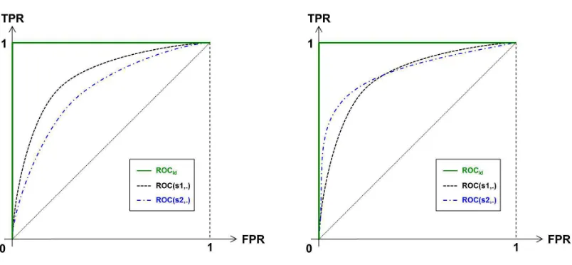
Definition 1 (TRUEROCCURVE)Let s be a scoring rule. The trueROCcurve of s is the “probability-probability” plot given by:

t∈R7→(P{s(X)>t|Y =−1},P{s(X)>t|Y =1})∈[0,1]2.

By convention, when a jump occurs in the plot of theROCcurve, the corresponding extremities of

the curve are connected by a line segment, so that theROCcurve of s can be viewed as the graph

of a continuous mappingα∈[0,1]7→ROC(s,α).

We refer to Cl´emenc¸on and Vayatis (2009c) for a list of properties of ROC curves (see the Appendix section therein). The ROC curve offers a visual tool for assessing ranking performance (see Figure 1): the closer to the left upper corner of the unit square [0,1]2 _{the curve ROC}₍_s_{, .}₎_, the better the scoring rule s. Therefore, the ROC curve conveys a partial order on the set of all

(4)

Figure 1: ROC curves.

scoring rules: for all pairs of scoring ruless1 ands2, we say thats2is more accurate thans1 when ROC(s1,α)≤ROC(s2,α) for all α∈[0,1]. By a standard Neyman-Pearson argument, one may establish that the most accurate scoring rules are increasing transforms of the regression function which is equal to the conditional probability functionηup to an affine transformation.

Definition 2 (OPTIMAL SCORING RULES)We call optimal scoring rules the elements of the set

S

∗ of scoring functions s∗such that∀(x,x′)∈

X

2_,_η₍_x₎_<_η₍_x′₎_⇒_s∗₍_x₎_<_s∗₍_x′₎_.

The fact that the elements of

S

∗ are optimizers of the ROC curve is shown in Cl´emenc¸on and Vayatis (2009c) (see Proposition 4 therein). When, in addition, the random variable η(X) is as-sumed to be continuous, then

S

∗coincides with the set of strictly increasing transforms ofη. The performance of a candidate scoring rulesis often summarized by a scalar quantity called theArea

Under the ROCCurve (AUC) which can be considered as a summary of the ROC curve. In the

paper, we shall use the following definition of the AUC.

Definition 3 (AUC)Let s be a scoring rule. TheAUCis the functional defined as:

AUC(s) =P{s(X1)<s(X2)|(Y1,Y2) = (−1,+1)}

+1

2P{s(X1) =s(X2)|(Y1,Y2) = (−1,+1)}, where(X1,Y1)and(X2,Y2)denote two independent copies of the pair(X,Y), for any scoring func-tion s.

(5)

statistical counterparts of ROC(s, .)and AUC(s)based on sampling data

D

n={(Xi,Yi): 1≤i≤n}

are obtained by replacing the class distributions by their empirical versions in the definitions. They are denoted byROC[(s, .)andAUC[(s)in the sequel.

Piecewise constant scoring rules. In the paper, we will focus on a particular subclass of scoring

rules.

Definition 4 (PIECEWISE CONSTANT SCORING RULE) A scoring rule s is piecewise constant if there exists a finite partition

P

of

X

such that for all

C

∈

P

, there exists a constant kC∈Rsuch that ∀x∈

C, s

(x) =kC.

This definition does not provide a unique characterization of the underlying partition. The partition

P

is minimal if, for any two of its elements

C

6=

C

′, we havekC 6=kC′. The scoring rule

conveys an ordering on the cells of the minimal partition.

Definition 5 (RANK OF A CELL)Let s be a scoring rule and

P

the associated minimal partition.

The scoring rule induces a rankingsover the cells of the partition. For a given cell

C

∈

P

, we

define its rank

R

s(

C

)∈ {1, . . . ,|

P

|}as the rank affected by the rankingsover the elements of the

partition. By convention, we set rank 1 to correspond to the highest score.

The advantage of the class of piecewise constant scoring rules is that they provide finite rankings on the elements of

X

and they will be the key for applying the aggregation procedure.

3. Aggregation of Scoring Rules

In recent years, the issue of summarizing or aggregating various rankings has been a topic of grow-ing interest in the machine-learngrow-ing community. This evolution was mainly motivated by practical problems in the context of internet applications: design of meta-search engines, collaborative filter-ing, spam-fightfilter-ing,etc. We refer for instance to Pennock et al. (2000), Dwork et al. (2001), Fagin et al. (2003) and Ilyas et al. (2002). Such problems have led to a variety of results, ranging from the generalization of the mathematical concepts introduced in social choice theory (see Barth´el´emy and Montjardet 1981 and the references therein) for defining relevant notions ofconsensusbetween rankings (Fagin et al., 2006), to the development of efficient procedures for computing such “con-sensus rankings” (Betzler et al., 2008; Mandhani and Meila, 2009; Meila et al., 2007) through the study of probabilistic models over sets of rankings (Fligner and Verducci , Eds.; Lebanon and Laf-ferty, 2003). Here we consider rank aggregation methods in the perspective of extending the bagging approach to ranking trees.

3.1 The Case of Piecewise Constant Scoring Rules

The ranking rules considered in this paper result from the aggregation of a collection of piecewise constant scoring rules. Since each of these scoring rules is related to a possibly different partition, we are lead to consider a collection of partitions of

X

. Hence, the aggregated rule needs to be defined on the least fine subpartition of this collection of partitions.

(6)

of nonempty subsets

C

⊂

X

which satisfy the following constraint : for all

C

∈

P

B, there exists

(

C

1, . . . ,

C

B)∈

P

1× · · · ×

P

Bsuch that

C

⊆

B

\

b=1

C

_b.

We denote

P

_B∗=T_b_≤_B

P

b.

One may easily see that

P

_B∗is a subpartition of any of the

P

b’s, and the largest one in the sense

that any partition

P

which is a subpartition of

P

_bfor allb∈ {1, . . . ,B}is a subpartition of

P

_B∗. The case where the partitions are obtained from a binary tree structure is of particular interest as we shall consider tree-based piecewise constant scoring rules later on. Incidentally, it should be noticed that, from a computational perspective, the underlying tree structures considerably help in getting the cells of

P

_B∗explicitly. We refer to Appendix D for further details.

Now consider a collection of piecewise constant scoring rulessb,b=1, . . . ,B, and denote their

associated (minimal) partitions by

P

_b. Each scoring rulesbnaturally induces a ranking (or a

pre-order) ∗

b on the partition

P

B∗. Indeed, for all (

C

,

C

′)∈

P

B∗2, one writes by definition

C

∗b

C

′

(respectively,

C

≺∗_b

C

′) if and only if

C

b ∗_b

C

_b′ (respectively,

C

b≺∗_b

C

_b′) where (

C

b,

C

_b′)∈

P

_b2 are

such that

C

×

C

′⊂

C

_b×

C

_b′.

The collection of scoring rules leads to a collection of B rankings on

P

_B∗. Such a collection is called aprofilein voting theory. Now, based on thisprofile, we would like to define a “central ranking” or aconsensus. Whereas the mean, or the median, naturally provides such a summary when considering scalar data, various meanings can be given to this notion for rankings (see Appendix B).

3.2 Probabilistic Measures of Scoring Agreement

The purpose of this subsection is to extend the concept of measures of agreement for rankings to scoring rules defined over a general space

X

which is not necessarily finite. In practice, however, we will only consider the case of piecewise constant scoring rules and we shall rely on the definition of the probabilistic Kendall tau.

Notations.We already introduced the notationsfor the preorder relation over the cells of a

parti-tion

P

as induced by a piecewise scoring rules. We shall use the ’curly’ notation for the preorder relation4_son

X

which is described through the following condition:∀

C

,

C

′∈

P

, we havex4_sx′, ∀x∈

C

,∀x′∈

C

′, if and only if

C

s

C

′. This is also equivalent tos(x)≤s(x′),∀x∈

C

,∀x′∈

C

′.

We now introduce a measure of similarity for preorders on

X

induced by scoring ruless1ands2. We recall here the definition of the theoretical Kendallτbetween two random variables.

Definition 7 (PROBABILISTIC KENDALLτ) Let(Z1,Z2)be two random variables defined on the

same probability space. The probabilistic Kendallτis defined as

τ(Z1,Z2) =1−2dτ(Z1,Z2), with:

dτ(Z1,Z2) =P{(Z1−Z′1)·(Z2−Z2′)<0}+ 1

2P{Z1=Z ′

1,Z26=Z2′} +1

2P{Z16=Z ′

(7)

where(Z₁′,Z₂′)is an independent copy of the pair(Z1,Z2).

As shown by the following result, whose proof is left to the reader, the Kendallτfor the pair (s(X),Y)is related to AUC(s).

Proposition 8 We use the notation p=P{Y =1}. For any real-valued scoring rule s, we have:

1

2(1−τ(s(X),Y)) =2p(1−p) (1−AUC(s)) + 1

2P{s(X)6=s(X

′₎_,_Y ₌_Y′_}_.

For given scoring ruless1ands2and considering the probabilistic Kendall tau for random vari-abless1(X) ands2(X), we can set: dX(s1,s2) =dτ(s1(X),s2(X)). One may easily check thatdX

defines a distance between the orderings4_s₁ and4_s₂ induced bys1 ands2 on the set

X

(which is supposed to coincide with the support of the distribution ofX). The following proposition shows that the deviation between scoring rules in terms of AUC is controlled by a quantity involving the probabilistic agreement based on Kendall tau.

Proposition 9 (AUCANDKENDALLτ) Assume p∈(0,1). For any scoring rules s1 and s2on

X

, we have:

|AUC(s1)−AUC(s2)| ≤

dX(s1,s2) 2p(1−p) =

1−τX(s1,s2) 4p(1−p) .

The converse inequality does not hold in general. Indeed, scoring rules with same AUC may yield to different rankings. However, the following result guarantees that a scoring rule with a nearly optimal AUC is close to the optimal scoring rules in the sense of Kendall tau, under the additional assumption that the noise condition introduced in Cl´emenc¸on et al. (2008) is fulfilled.

Proposition 10 (KENDALLτAND OPTIMALAUC)Assume that the random variableη(X)is con-tinuous and that there exist c<∞and a∈(0,1)such that:

∀x∈

X

, _E|η(X)−η(x)|−a_≤_c_. ₍₁₎

Then, we have, for any scoring rule s and any optimal scoring rule s∗∈

S

∗:

1−τX(s∗,s)≤C·(AUC∗−AUC(s))a/(1+a) ,

with C=3·c1/(1+a)·(2p(1−p))a/(1+a)_.

Remark 11 (ON THE NOISE CONDITION) As shown in previous work, the condition (1) is rather weak. Indeed, it is fulfilled for any a∈(0,1) as soon the probability density function ofη(X) is bounded (see Corollary 8 in Cl´emenc¸on et al. 2008).

The next result shows the connection between the Kendall tau distance between preorders on

X

induced by piecewise constant scoring ruless1ands2and a specific notion of distance between the rankingss1 ands2 on

P

.

Lemma 12 Let s1, s2, two piecewise constant scoring rules. We have: dX(s1,s2) =2

∑

1≤k<l≤K

(8)

where, for two orderings,′_{on a partition of cells}_{_C

k : k=1, . . . ,K}, we have:

Uk,l(,′) =I{(

R

(

C

k)−

R

(

C

l))(

R

′(

C

_k)−

R

′(

C

_l))<0}

+1

2I{

R

(

C

k) =s(

C

l),

R

′(

C

k)6=

R

′(

C

l)} +1

2I{

R

′(

C

k) =

R

′(

C

l),

R

(

C

k)6=

R

(

C

l)}. The proof is straightforward and thus omitted.

Notice that the termUk,l(s1,s2)involved in Equation (2) is equal to 1 when the cells

C

kand

C

lare not sorted in the same order bys1ands2(in absence of ties), to 1/2 when they are tied for one ranking but not for the other, and to 0 otherwise. As a consequence, the agreementτX(s1,s2)may be viewed as a “weighted version” of the rate of concordant pairs of the cells of

P

measured by the classical Kendallτ(see the Appendix B). A statistical version ofτX(s1,s2)is obtained by replacing the values ofµ(

C

_k)by their empirical counterparts in Equation (2). We thus set:

bτX(s1,s2) =1−2dbX(s1,s2), (3) wheredbX(s1,s2) =2/(n(n−1))∑i<jK(Xi,Xj) is aU-statistic of degree 2 with symmetric kernel

given by:

K(x,x′) =I{(s1(x)−s1(x′))·(s2(x)−s2(x′))<0}+ 1

2I{s1(x) =s1(x ′₎_,_s

2(x)6=s2(x′)} +1

2I{s1(x)6=s1(x ′₎_,_s

2(x) =s2(x′)}. Remark 13 Other measures of agreement between4_s₁ and4_s₂ could be considered alternatively. For instance the definitions previously stated can easily be extended to the Spearman correlation coefficientρX(s1,s2)(see Appendix B), that is the linear correlation coefficient between the random variables Fs1(s1(X))and Fs2(s2(X)), where Fsi denotes the cdf of si(X), i∈ {1,2}.

3.3 Median Rankings

The method for aggregating rankings we consider here relies on the so-calledmedian procedure, which belongs to the family of metric aggregation procedures (see Barth´el´emy and Montjardet 1981 for further details). Letd(., .)be some metric or dissimilarity measure on the set of rankings on a finite set

Z

. By definition, a median rankingamong a profile Π={k: 1≤k≤K} with

respect todis any rankingmedon

Z

that minimizes the sum∆Π()

de f

= ∑Kk=1d(,k)over the set

R(

Z

)of all rankingson

Z

:

∆Π(med) = min

: ranking onZ∆Π().

Notice that, when

Z

is of cardinalityN<∞, there are

#R(

Z

) =

N

∑

k=1

(−1)k k

∑

m=1

(−1)m

k m

mN

(9)

combinatorial optimization problems (see Wakabayashi 1998, Hudry 2004, Hudry 2008 and the references therein). It is worth noticing that a median ranking is far from being unique in general. One may immediately check for instance that any ranking among the profile made of all rankings on

Z

={1,2}is a median in Kendall sense, that is, for the metricdτ. From a practical perspective, ac-ceptably good solutions can be computed in a reasonable amount of time by means of metaheuristics such as simulated annealing, genetic algorithms or tabu search (see Spall 2003). The description of these computational aspects is beyond the scope of the present paper (see Charon and Hudry 1998 or Laguna et al. 1999 for instance). We also refer to recent work in Klementiev et al. (2009).

When it comes to preorders on a set

X

of infinite cardinality, defining a notion of aggregation becomes harder. Given a pseudo-metric such as dτ andB≥1 scoring rules s1, . . . , sB on

X

, the

existence of ¯sin

S

such that∑Bb=1dτ(s¯,sb) =mins∑Bb=1dτ(s,sb)is not guaranteed in general.

How-ever, when considering piecewise constant scoring rules with corresponding finite subpartition

P

of

X

, the corresponding preorders are in one-to-one correspondence with rankings on

P

and the minimum distance is thus effectively attained.

Aggregation of piecewise constant scoring rules. Consider a finite collection of piecewise constant

scoring rulesΣB={s1, . . . ,sB}on

X

, withB≥1.

Definition 14 (TRUE MEDIAN SCORING RULE). Let

S

be a collection of scoring rules. We calls¯B

amedian scoring ruleforΣBwith respect to

S

if

¯

sB=arg min s∈S

∆B(s),

where∆B(s) =∑Bb=1dX(s,sb)for s∈

S

.

The empirical median scoring rule is obtained in a similar way, but the true distance dX is

replaced by its empirical counterpartd_b_τ_X, see Equation (3).

The ordinal approach.Metric aggregation procedures are not the only way to summarize a profile of

rankings. The so-called “ordinal approach” provides a variety of alternative techniques for combin-ing rankcombin-ings (or, more generally, preferences), returning to the famous “Arrow’s voting paradox”. The ordinal approach consists of a series of duels (i.e., pairwise comparisons) as in Condorcet’s method or successive tournaments as in the proportional voting Hare system, see Fishburn (1973). Such approaches have recently been the subject of a good deal of attention in the context of

pref-erence learning(also referred to as methods forranking by pairwise comparison, see H¨ullermeier

et al. 2008 for instance).

Ranks vs. Rankings. LetΣB={s1, . . . , sB},B≥1, be a collection of piecewise constant scoring

rules andX′(m)={X₁′, . . . ,X_m′} a collection ofm≥1 i.i.d. copies of the input variable X. When it comes to rank the observationsX_i′“consensually”, two strategies can be considered: (i) compute a “median ranking rule” based on theB rankings of the cells for the largest subpartition and use it for ranking the new data as previously described, or (ii) compute, for each scoring rulesb, the

(10)

collectionΣBis obtained from training data

D

n. The difference between (i) and (ii) is that (i) does

not use the data to be rankedX′(m) but only relies on training data

D

n. However, when both the

size of the training sample

D

nand of the test data setX′(m)are large, the two approaches lead to the

optimization of related quantities.

4. Consistency of Aggregated Scoring Rules

We now provide statistical results for the aggregated scoring rules in the spirit of random forests (Breiman, 2001). In the context of classification, consistency theorems were derived in Biau et al. (2008). Conditions for consistency of piecewise constant scoring rules have been studied in Clémençon and Vayatis (2009c) and Clémençon et al. (2011). Here, we address the issue of AUC consistency of scoring rules obtained as medians over a profile of consistent randomized scoring rules for the (probabilistic) Kendallτdistance. Arandomized scoring ruleis a random element of the form_bsn(·,Z), depending on both the training sample

D

n={(X1,Y1), . . . , (Xn,Yn)} and a

ran-dom variableZ, taking values over a measurable space

Z

, independent of

D

_n, which describes the randomization mechanism.

The AUC of a randomized scoring rule_bsn(·,Z)is given by:

AUC(_bsn(·,Z)) =P{bsn(X,Z)<bsn(X′,Z)|(Y,Y′) = (−1,+1)}

+1

2P{bsn(X,Z) =bsn(X

′_,_Z₎_|₍_Y_,_Y′_{) = (}₋₁_,₊₁₎_}_,

where the conditional probabilities are taken over the joint probability of independent copies(X,Y) and(X,Y′)andZ, given the training data

D

n.

Definition 15 (AUC-CONSISTENCY)The randomized scoring rule_bsnis said to beAUC-consistent

(respectively, stronglyAUC-consistent) when the convergence

AUC(_bsn(·,Z))→AUC∗asn→∞,

holds in probability (respectively, almost-surely).

LetB≥1. Given

D

n, one may drawBi.i.d. copiesZ1, . . . , ZBofZ, yielding the collectionΣbB

of scoring rules_bsn(·,Zj), 1≤ j≤B. Let

S

be a collection of scoring rules and suppose that ¯sBis a

median scoring rulefor the profileΣbBwith respect to

S

in the sense of Definition 14. The next result

shows that AUC-consistency is preserved for a median scoring rule of AUC-consistent randomized scoring rules.

Theorem 16 (CONSISTENCY AND AGGREGATION) Set B≥1. Consider a class

S

of scoring rules. Assume that:

• the assumptions on the distribution of(X,Y)in Proposition 10 are fulfilled.

• the randomized scoring rule_bsn(·,Z)isAUC-consistent (respectively, stronglyAUC-consistent).

• for all n,B≥1, and for any sample

D

n, there exists a median scoring rules¯B∈

S

for the

(11)

• we have

S

∗∩

S

6= /0.

Then, the aggregated scoring rules¯BisAUC-consistent (respectively, stronglyAUC-consistent).

We point out that the last assumption which states that the class

S

of candidate median scoring rules contains at least one optimal scoring function can be removed at the cost of an extra bias term in the rate bound. Consistency results are then derived by picking the median scoring rule, for eachn, in a class

S

_n such that there exists a sequence ˜sn∈

S

nwhich fulfills AUC(˜sn)→AUC∗as

n→∞. This remark covers the special case where_bsn(·,Z)is a piecewise constant scoring rule with

a range of cardinalitykn↑∞and the median is taken over the set

S

nof scoring functions with range

of cardinality less thank_nB. The bias is then of order 1/k_n2B under mild smoothness conditions on ROC∗, as shown by Proposition 7 in Cl´emenc¸on and Vayatis (2009b).

From a practical perspective, median computation is based on empirical versions of the proba-bilistic Kendallτinvolved (see Equation (3)). The following result shows the existence of scoring rules that are asymptotically median with respect todX, provided that the class

S

over which the

median is computed is not too complex. Here we formulate the result in terms of a VC major class of functions of finite dimension (see Dudley 1999 for instance). We first introduce the following notation, for anys∈

S

:

b

∆B,m(s) = B

∑

j=1

b

dX(s,sj),

where the estimatedbX ofdX is based onm≥1 independent copies ofX.

Theorem 17 (EMPIRICAL MEDIAN COMPUTATION) Fix B≥1. LetΣB={s1, . . . ,sB}be a finite

collection scoring rules and

S

a class of scoring rules which is a VC major class. We consider the

empirical median scoring rule_esm=arg mins∈S∆bB,m(s). Then, as m→∞, we have

∆B(esm)→min

s∈S ∆B(s)with probability one.

The empirical aggregated scoring rule we consider in the next result relies on two data samples. The training sample

D

n, completed by the randomization onZ, leads to a collection of scoring rules

which are instances of the randomized scoring rule. Then a sampleX′(m)={X₁′, . . . ,X_m′} is used to compute the empirical median. Combining the two preceding theorems, we finally obtain the consistency result for the aggregated scoring rule.

Corollary 18 Fix B≥1and

S

a VC major class of scoring rules. Consider a training sample

D

n

of size n with i.i.d. copies of(X,Y)and a sampleX′(m)of size m with i.i.d. copies of X . We consider the collectionΣbB of randomized scoring rules bsn(·,Zj) in

S

built out of

D

n and we introduce the

empirical median ofbΣB with respect to

S

obtained by using the test setX′(m). We denote this fully

empirical median scoring rule bysbn,m. If the assumptions of Theorem 16 are satisfied, then we have:

AUC(s_bn,m) P

−

→AUC∗asn,m→∞.

The results stated above can be extended to any median scoring rule based on a pseudo-metric d on the set of preorders on

S

which is equivalent todX, that is, such thatc1dX ≤d ≤c2dX, with

(12)

5. Ranking Forests

In this section, we introduce an implementation of the principles described in the previous sections for the aggregation of scoring rules. Here we focus on specific piecewise constant scoring rules based on ranking trees (Clémençon and Vayatis, 2009c; Clémençon et al., 2011). We propose var-ious schemes for randomizing the features of these trees. We eventually describe the RANKING

FORESTalgorithm which extends to bipartite ranking the celebrated RANDOMFORESTSalgorithm (Breiman, 1996; Amit and Geman, 1997; Breiman, 2001).

5.1 Tree-structured Scoring Rules

We consider piecewise constant scoring rules which can be represented in a left-right oriented binary tree. We recall that, in the context of classification, decision trees are very useful as they offer the possibility of interpretation for the selected classification rule. In the presence of classification data, one may entirely characterize a classification rule by means of a partition

P

of the input space

X

and a training set

D

_n={(Xi,Yi): 1≤i≤n}of i.i.d. copies of the pair(X,Y)through amajority

voting scheme. Indeed, a new instance x∈

X

would receive the label corresponding to the most

frequent one among the data pointsXiwithin the cell

C

∈

P

such thatx∈

C

. However, in bipartite

ranking, the notion of local majority vote makes no sense since the ranking problem is of global nature. As a matter of fact, the issue is to rank the cells of the partition with respect to each other. It is assumed that ties among the ordered cells can be observed in the subsequent analysis and the usualMID-RANKconvention is adopted. We refer to the Appendix A for a rigorous definition of the notion ofrankingin the case of ties. We also point out that the termpartial rankingis often used in this context (see Diaconis 1989, Fagin et al. 2006).

By restricting the search of candidates to the collection of piecewise constant scoring rules, the learning problem boils down here to finding a partition

P

={

C

k}1≤k≤K of

X

, with 1≤K <∞,

together with a rankingP of the

C

k’s (i.e., a preorder on

P

), so that the ROC curve of the scoring

rule given by

sP,P(x) =

K

∑

k=1

(K−

R

_P(

C

k) +1)·I{x∈

C

k}

be as close as possible of ROC∗, where

R

P(

C

k)denotes the rank of

C

k, 1≤k≤K, among all cells

of

P

according toP.

We now describe such scoring rules in the case where the partition arises from a tree structure. For such a partition, a ranking of the cells can be simply defined by equipping the tree with a left-right orientation. In order to describe how a ranking tree can be built so as to maximize AUC, further concepts are required. Bymaster ranking tree

T

_D, here we mean a complete, left-right oriented, rooted binary tree with depthD≥1. At depthd=0, the entire input space

C

0,0=

X

forms its root. Every non terminal node(d,k), with 0≤d<Dand 0≤k<2d, is in correspondence with a subset Cd,k⊂

X

, and has two siblings, each one corresponding to a subcell obtained by splittingCd,k: the

left sibling Cd+1,2kis related to the leaf(d+1,2k), while theright sibling Cd+1,2k+1=Cd,k\Cd+1,2k

is related to the leaf(d+1,2k+1)in the tree structure. We point out that an asymmetry is introduced at this point as the left sibling is assumed to have a lower rank (or higher score) than the right sibling in the ranking of the partition’s cells. With this convention, it is easy to use any subtree

T

⊂

T

D

(13)

related to the scoring rule defined by: ∀x∈

X

,

sT(x) =

∑

(d,k): terminal node ofT

(2D−2D−dk)·I{x∈Cd,k}.

The score valuesT(x)can be computed in a top-down manner, using the underlying “heap” struc-ture. Starting from the initial value 2D at the root node, at each subsequent inner node (d,k), 2D−(d+1)is subtracted to the current value of the score if xmoves down to the right sibling(d+ 1,2k+1), whereas one leaves the score unchanged ifxmoves down to the left sibling. The proce-dure is depicted in Figure 2.

Figure 2: Ranking tree - the ranks can be read on the leaves of the tree from left (8 is the highest rank/score) to right (1 corresponds to the smallest rank/score). In case of a pruned tree (such as the one with leaves taken to be the shaded nodes), the orientation is conserved.

5.2 Feature Randomization inTREERANK

The concept ofbagging(forbootstrapaggregatingtechnique) was introduced in Breiman (1996). The major novelty in the RANDOMFORESTmethod (Breiman, 2001) consisted in randomizing the

features used for recursively splitting the nodes of the classification/regression trees involved in the committee-based prediction procedure. Our reference method for aggregating tree-based scoring rules is the TREERANKprocedure (we refer to the Appendix and the papers Cl´emenc¸on and Vayatis

(14)

classifier is chosen to be a decision tree, this permits an additional randomization step. We thus propose two possible feature randomization schemesFT for TREERANKandFLfor LEAFRANK.

FT: At each node(d,k) of the master ranking tree

T

D, draw at random a set of q0≤q indexes

{i1, . . . ,iq0} ⊂ {1, . . . ,q}. Implement the LEAFRANK splitting procedure based on the de-scriptor(X(i1)_{, . . . ,}_X(iq0))to split the cell C_d_,_k.

FL: For each node(d,k)of the master ranking tree

T

D, at each node of the cost-sensitive

clas-sification tree describing the split of the cell

C

_d_,_k into two children, draw at random a set of q1≤q indexes{j1, . . . ,jq1} ⊂ {1, . . . ,q}and perform an axis-parallel cut using the descriptor

(X(j1)_{, . . . ,}_X(jq1)).

We underline that, of course, the randomization strategyFT can be applied to the TREERANK

algorithm whatever the classification technique chosen for the splitting step. In addition, when the latter is itself a tree-based method, these randomization procedures do not exclude each other. At each node(d,k)of the ranking tree, one may first draw at random a collection

F

d,k ofq0features and then, when growing the cost-sensitive classification tree describingCd,k’s split, divide each node

based on a sub-collection ofq1≤q0features drawn at random among

F

d,k.

5.3 TheRANKINGFORESTAlgorithm

Now that the rationale behind the RANKING FOREST procedure has been given, we describe its successive steps in detail. Based on a training sample

D

_n={(X1,Y1), . . . ,(Xn,Yn)}, the algorithm is

performed in three stages, as follows.

RANKINGFOREST

1. Parameters. Bnumber of bootstrap replicates, n∗ bootstrap sample size, TREERANK

tuning parameters (depthDand presence/absence of pruning),(FT,FL)feature

random-ization strategy,d pseudo-metric.

2. Bootstrap profile makeup.

(a) (RESAMPLING STEP.) Build B independent bootstrap samples

D

₁∗, . . . ,

D

_B∗, by

drawing with replacementn∗·Bpairs among the original training sample

D

n.

(b) (RANDOMIZEDTREERANK.) Forb=1, . . . , B, run TREERANKcombined with

the feature randomization method (FT,FL)based on the sample

D

_b∗, yielding the

ranking tree

T

_b∗, related to the partition

P

_b∗of the space

X

.

3. Aggregation. Compute the largest subpartition partition

P

∗=TB_b₌₁

P

_b∗. Let∗_bbe the ranking of the cells of

P

∗induced by

T

_b∗,b=1, . . . , B. Compute a median ranking∗ related to the bootstrap profile Π∗₌_{∗

b: 1≤b≤B} with respect to the metricd on

R(

P

∗):

∗=arg min ∈R(P∗₎

dΠ∗(),

(15)

Remark 19 (ON TUNING PARAMETERS.) As mentioned in 3.3, aggregating ranking rules is com-putationally expensive. The empirical results displayed in Section 6 suggest to aggregate several dozens of randomized ranking trees of moderate, or even small, depth built from bootstrap samples of size n∗≤n.

Remark 20 (“PLUG-IN” BAGGING.) As pointed out in Cl´emenc¸on and Vayatis (2009c) (see

Re-mark 6 therein), given an ordered partition(

P

,

R

P)of the feature space

X

, a “plug-in” estimate of

the (optimal scoring) function S=Hη◦ηcan be automatically deduced from any ordered partition

(or piecewise constant scoring rule equivalently) and the data

D

n, where Hη denotes the

condi-tional cdf ofη(X)given Y =−1. This scoring rule is somehow canonical in the sense that, given

Y =−1, H(X)is distributed as a uniform r.v. on[0,1], with H being the conditional distribution

of X . Considering a partition

P

={

C

k}1≤k≤K equipped with a ranking

R

P, the plug-in estimate is

given by

b

SP,RP(x) =

K

∑

k=1

b

α(Rk)·I{x∈

C

k}, x∈

X

,

where Rk=Sl:R(k)≤R(l)Cl. Notice that, as a scoring rule,SbP,RP yields the same ranking as sP,RP,

provided thatαb(

C

k)>0for all k=1, . . . ,K. Adapting the idea proposed in Section 6.1 of Breiman

(1996) in the classification context, an alternative to the rank aggregation approach proposed here naturally consists in computing the average of the piecewise-constant scoring rulesSe∗_T∗

b thus defined

by the bootstrap ranking trees and consider the rankings induced by the latter. This method we call “plug-in bagging” is however less effective in many situations, due to the inaccuracy/variability of the probability estimates involved.

Ranking stability. LetΘ=

X

× {−1,+1}. From the view developed in this paper, a ranking

algo-rithm is a functionSthat maps any data sample

D

n∈Θn,n≥1, to a scoring rulebsn. In the ranking

context, we will say that a learning algorithm is “stable” when the preorder on

X

it outputs is not much affected by small changes in the training set. We propose a natural way of measuring ranking (in)stability, through the computation of the following quantity:

Instabn(S) =E dX bsn,bs′n

, (4)

where the expectation is taken over two independent training samples

D

nand

D

n′, both made ofn

i.i.d. copies of the pair(X,Y), and_bsn=S(

D

n),bs′n=S(

D

n′). Incidentally, we highlight the fact that

the bootstrap stage of RANKINGFORESTcan be used for assessing the stability of the base ranking algorithm. Indeed, set_bs(_nb∗)=S(

D

_b∗)andsb(

b′)

n∗ =S(

D

_b∗′)obtained from two bootstrap samples. Then,

the quantity:

\ Instabn(S) =

2

B(B−1)_1≤_b

∑

_<_b′_≤_B

b

dX

b

s(_nb∗),sb(b ′₎

n∗

,

can be possibly interpreted as a bootstrap estimate of (4).

We finally underline that the outputs of the RANKINGFORESTcan also be used for monitoring

(16)

6. Numerical Experiments

The purpose of this section is to measure the impact of aggregation with resampling and feature randomization on the performance of the TREERANK/LEAFRANKprocedure.

Data sets. We have considered artificial data sets where class-conditional distributions ofX goven

Y =±1 are gaussian in dimensions 10 and 20. Three examples are considered here:

• RF 10 - class-conditional distributions have the same means (µ+ =µ−=0) but different

covariance matrices (Σ+=Id10andΣ−=1.023·Id10); optimal AUC is AUC∗=0.76;

• RF 20- class-conditional distributions have different mean vectors (||µ+−µ−||=0.9) and

covariance matrices (Σ+=Id20andΣ−=1.23·Id20); optimal AUC is AUC∗=0.77;

• RF 10 sparse- class-conditional distributions have a 6-dimensional marginal distribution in

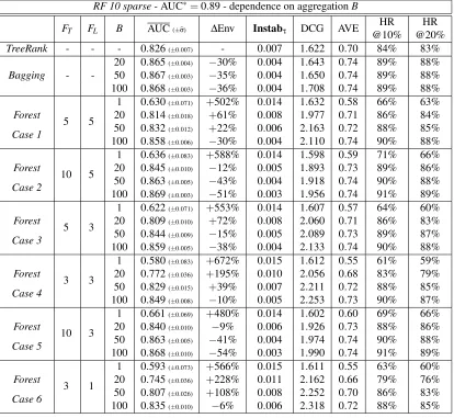
common, and the regression functionη(x)depends on four components of the input vectorX onlyoptimal AUC is AUC∗=0.89.

With these data sets, the series of experiments below capture the influence on ranking performance of separability, dimension, and sparsity.

Sample sizes. In order to quantify the impact of bagging and random feature selection on the

accu-racy/stability of the resulting ranking rule, the algorithm has been run under various configurations for each data set on 30 independent training samples for each sample size ranging fromn=250 to n=3000. The test sample was taken of size 3000 in all experiments.

Variants ofTREERANKand parameters.In the intensive comparisons we have performed, we have

considered the following variants:

• Plain TREERANK/LEAFRANK- in this version, all input dimensions are involved in the split-ting stage; the maximum depth of the master ranking tree is 10, and the maximum depth of the ranking tree using orthogonal splits in the LEAFRANKprocedure is 8 for the use caseRF

10 sparseand also 10 for the two others.

• BAGGING RANKING TREES - thebagging version uses the plain TREERANK/LEAFRANK

as described above with bootstrap samples of sizeB=20,B=50, andB=100.

• RANKINGFORESTS- the forestversion involves additional parameters for feature random-ization which can affect both the master ranking tree (FT for TREERANK) and the splitting

rule (FLfor LEAFRANK); these parameters indicate the number of dimensions randomly

cho-sen along which the best split is chocho-sen ; we have tried six different sets of parameters (Cases 1 to 6) whereFT takes values 3, 5, and 10 (or 20 for the data setRF 20), andFLtakes values

1, 3, and 5 (plus 10 for the data setRF 20); bootstrap samples are chosen of sizeB=1 (single tree with feature randomization),B=20,B=50, andB=100.

In the case of bagging and forests, aggregation is performed by taking the pointwise median value of ranks for the collection of ranking trees which have been estimated on each bootstrap sample. This choice allows for very fast evaluations of the aggregated scoring rule (see the last paragraph of Section 3.3 for a justification).

Performance. For each variant and each set of parameters and sample size, we performed 30

(17)

• AUC andσ_b2 _{- Average AUC and standar type error are computed based on the test sample} results over the 30 replications;

• ∆Env - this indicator quantifies the accuracy of the variant through the relative improvement of the envelope on the ROC curve over the 30 replications compared to the plain TREE

R-ANK/LEAFRANK(e.g., if∆Env=−30% for BAGGINGit means that the envelope of the ROC curve is 30% narrower than with TREERANK); the more negative the better the performance accuracy;

• Instabτ- Instability measure applied to the ranking algorithm (e.g., Ranking Forest), estimate of (4), which reproduces the quantityInstab\n(S)using the Kendalτas a distance; the smaller

the quantity the more stable the method;

• DCG and AVE - theDiscounted Cumulative Gain and theAverage Precisionprovide mea-sures which are sensitive to the top ranked instances; they can both be expressed as conditional linear rank statistics (see Clémençon and Vayatis 2007 and Clémençon and Vayatis 2009a) with score-generating function given by 1/(ln(1+x))(DCG) or 1/x(AP);

• HR@u% - theHit Ratioatu% is a relative count of positive instances among a proportionu of best scored instances.

These indicators capture the most important properties as far as quality assessment for scoring rules is concerned: average and local performance, stability of the rule, accuracy of ROC performance.

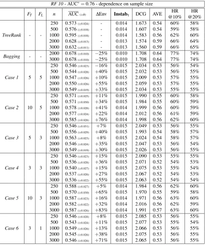
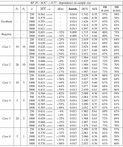
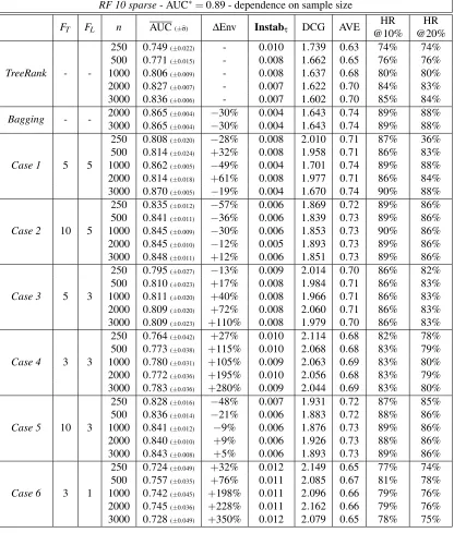
Results and comments. Results are collected in a series of Tables 1, 2, 3, 4, 5, 6. We also report

enveloppes on ROC curves over the series of replications of the experiments with the same parame-ters (see Figures 3 and 4). We study in particular the impact of mixed effects of randomization with sample size (Tables 1, 2, 3) or aggregation (Tables 4, 5, 6). Our main observations are the following:

• The sample size of the training set has a moderate impact on performance of RANKING

FORESTwhile it helps significantly single trees in the plain TREERANK;

• In the case of small sample sizes, RANKINGFORESTwith little randomization (Cases 2 and 5) boost performance compared to the plain TREERANK;

• Increasing the amount of aggregation always improves performance and accuracy except in some situations in the non-sparse data sets (little randomizationFT=d,Blarge);

• BAGGINGwithB=20 ranking trees already improves plain TREERANKdramatically;

• Randomization reveals its power in the sparse data set; when all input variables are relevant, highly randomized strategies (Cases 4 and 6) may fail to capture good scoring rules unless a large amount of ranking trees are aggregated (Babove 50).

(18)

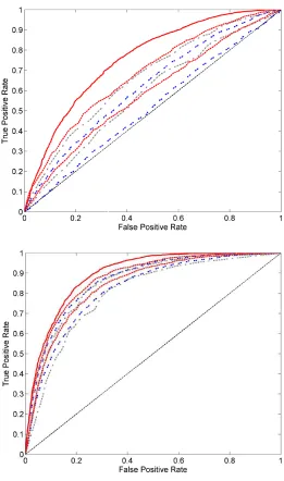
Figure 3: Comparison of envelopes on ROC curves - Results obtained with RANKING FORESTS

withB=50 (blue, double dashed) and 100 (red, solid, dashed). The upper display shows results on the data setRF 10while the lower display corresponds to the curves obtained on the data setRF 10 sparse. RANKINGFORESTSused correspond to Case 3, training size is 2000, and optimal ROC curve is in thick red.

7. Conclusion

The major contribution of the paper was to show how to apply the principles of the RANDOMFOR

(19)

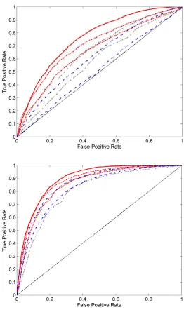
Figure 4: Comparison of envelopes on ROC curves - Results obtained with BAGGING(red, solid

and dashed) and RANKING FORESTS (blue, double dashed) with B=50. The upper display shows results on the data setRF 10while the lower display corresponds to the curves obtained on the data setRF 10 sparse. RANKINGFORESTSused correspond to

Case 3, training size is 2000, and optimal ROC curve is in thick red.

(20)

back-RF 10- AUC∗=0.756 - dependence on aggregation

FT FL B AUC(±σb) ∆Env Instab_τ DCG AVE HR HR

@10% @20%

TreeRank - - - 0.628(±0.013) - 0.013 1.574 0.59 66% 64%

Bagging -

-20 0.678(±0.010) −25% 0.010 1.708 0.64 77% 74% 50 0.686(±0.008) −29% 0.009 1.745 0.64 78% 74% 100 0.689(±0.009) −29% 0.009 1.819 0.65 78% 74% 1 0.508(±0.027) +65% 0.016 1.563 0.50 49% 50%

Forest

5 5 20 0.550(±0.026) +55% 0.015 2.059 0.53 57% 55%

Case 1 50 0.567(±0.025) +46% 0.015 2.210 0.55 59% 57%

100 0.642(±0.016) −7% 0.011 2.288 0.61 71% 67% 1 0.525(±0.025) +68% 0.015 1.564 0.51 52% 52%

Forest

10 5 20 0.577(±0.024) +22% 0.014 2.012 0.56 61% 59%

Case No. 2 50 0.615(±0.020) +21% 0.013 2.187 0.58 67% 64%

100 0.585(±0.025) +34% 0.014 2.357 0.56 62% 60% 1 0.512(±0.024) +61% 0.016 1.564 0.50 49% 49%

Forest

5 3 20 0.546(±0.024) +35% 0.015 2.047 0.53 56% 54%

Case 3 50 0.577(±0.025) +35% 0.014 2.215 0.56 61% 59%

100 0.648(±0.019) +23% 0.011 2.294 0.61 72% 68% 1 0.512(±0.023) +51% 0.015 1.570 0.50 47% 49%

Forest

3 3 20 0.537(±0.026) +27% 0.015 2.067 0.52 54% 53%

Case 4 50 0.563(±0.028) +42% 0.015 2.249 0.54 58% 57%

100 0.595(±0.019) 0% 0.014 2.345 0.57 64% 61% 1 0.516(±0.029) +95% 0.016 1.564 0.51 51% 51%

Forest

10 3 20 0.582(±0.022) +32% 0.014 2.016 0.56 62% 59%

Case 5 50 0.616(±0.022) +11% 0.013 2.161 0.59 67% 64%

100 0.579(±0.023) +30% 0.014 2.423 0.56 61% 59% 1 0.517(±0.028) +81% 0.016 1.567 0.51 51% 52%

Forest

3 1 20 0.545(±0.026) +38% 0.015 2.075 0.53 56% 55%

Case 6 50 0.565(±0.024) +28% 0.015 2.224 0.55 59% 57%

100 0.647(±0.016) +3% 0.011 2.306 0.61 70% 67%

Table 1: Comparison of TREERANK/LEAFRANKand BAGGINGwith RANKING FORESTS - Im-pact of randomization(FT,FL)and resampling with aggregation(B)on the data setRF 10

with training sample sizen=2000.

ground theory for ranking rule aggregation. Encouraging experimental results based on artificial data have also been obtained, demonstrating how bagging combined with feature randomization may significantly enhance ranking accuracy and stability both at the same time. Truth be told, the-oretical explanations for the success of RANKINGFORESTin these situations are left to be found.

(21)

RF 20- AUC∗=0.773 - dependence on aggregation

@10% @20%

TreeRank - - - 0.613(±0.013) - 0.013 1.614 0.59 67% 64%

Bagging - - 20 0.691(±0.009) −32% 0.009 1.715 0.66 80% 75% 50 0.699(±0.006) −43% 0.008 1.816 0.66 81% 76% 1 0.534(±0.033) +120% 0.015 1.599 0.53 56% 56%

Forest

10 10 20 0.623(±0.028) +78% 0.013 2.017 0.60 68% 65%

Case 1 50 0.667(±0.021) +33% 0.011 2.017 0.63 73% 70%

100 0.726(±0.011) −25% 0.007 2.160 0.67 80% 77% 1 0.551(±0.033) +114% 0.015 1.599 0.54 58% 57%

Forest

20 10 20 0.673(±0.019) +28% 0.011 1.989 0.64 73% 70%

Case 2 50 0.706(±0.012) −15% 0.009 2.104 0.66 77% 74%

100 0.693(±0.014) 0% 0.009 2.250 0.65 76% 73% 1 0.534(±0.030) +100% 0.015 1.599 0.53 56% 55%

Forest

10 5 20 0.625(±0.025) +64% 0.013 2.077 0.60 68% 65%

Case 3 50 0.675(±0.013) −6% 0.011 2.179 0.64 75% 71%

100 0.726(±0.009) −35% 0.007 2.171 0.67 80% 77% 1 0.516(±0.038) +138% 0.016 1.599 0.52 53% 53%

Forest

5 5 20 0.585(±0.030) +93% 0.014 2.050 0.57 63% 61%

Case 4 50 0.625(±0.026) +50% 0.013 2.217 0.60 67% 65%

100 0.702(±0.013) −16% 0.009 2.247 0.66 78% 74% 1 0.547(±0.034) +123% 0.015 1.598 0.54 58% 56%

Forest

20 5 20 0.666(±0.020) +25% 0.011 2.007 0.63 74% 70%

Case 5 50 0.705(±0.011) −23% 0.009 2.128 0.66 78% 74%

100 0.658(±0.021) +24% 0.011 2.329 0.62 71% 69% 1 0.510(±0.040) +157% 0.016 1.597 0.51 52% 52%

Forest

5 1 20 0.574(±0.035) +97% 0.015 2.120 0.56 61% 59%

Case 6 50 0.614(±0.027) +64% 0.014 2.238 0.59 67% 64%

100 0.710(±0.011) −19% 0.009 2.261 0.66 78% 75%

with training sample sizen=2000.

Appendix A. Axioms for Ranking Rules

Throughout this paper, we call arankingof the elements of a set

Z

anytotal preorderon

Z

, that is, a binary relationfor which the following axioms are checked.

1. (TOTALITY) For all(z1,z2)∈

Z

2, eitherz1z2or elsez2z1holds. 2. (TRANSITIVITY) For all(z1,z2,z3): ifz1z2andz2z3, thenz1z3.

(22)

RF 10 sparse- AUC∗=0.89 - dependence on aggregationB

@10% @20%

TreeRank - - - 0.826(±0.007) - 0.007 1.622 0.70 84% 83%

Bagging -

-20 0.865(±0.004) −30% 0.004 1.643 0.74 89% 88% 50 0.867(±0.003) −35% 0.004 1.650 0.74 89% 88% 100 0.868(±0.003) −36% 0.004 1.708 0.74 89% 88% 1 0.630(±0.071) +502% 0.014 1.632 0.58 66% 63%

Forest

5 5 20 0.814(±0.018) +61% 0.008 1.977 0.71 86% 84%

Case 1 50 0.832(±0.012) +22% 0.006 2.163 0.72 88% 85%

100 0.858(±0.006) −30% 0.004 2.110 0.74 90% 88% 1 0.636(±0.083) +588% 0.014 1.598 0.59 71% 66%

Forest

10 5 20 0.845(±0.010) −12% 0.005 1.893 0.73 89% 86%

Case 2 50 0.863(±0.005) −43% 0.004 1.918 0.74 90% 88%

100 0.869(±0.003) −51% 0.003 1.956 0.74 91% 89% 1 0.622(±0.071) +553% 0.014 1.607 0.57 64% 60%

Forest

5 3 20 0.809(±0.010) +72% 0.008 2.060 0.71 86% 83%

Case 3 50 0.844(±0.009) −15% 0.005 2.089 0.73 89% 87%

100 0.859(±0.005) −38% 0.004 2.133 0.74 90% 88% 1 0.580(±0.083) +672% 0.015 1.612 0.55 61% 59%

Forest

3 3 20 0.772(±0.036) +195% 0.010 2.056 0.68 83% 79%

Case 4 50 0.829(±0.015) +39% 0.007 2.211 0.72 88% 85%

100 0.849(±0.008) −10% 0.005 2.253 0.73 90% 87% 1 0.661(±0.069) +480% 0.014 1.602 0.60 69% 66%

Forest

10 3 20 0.840(±0.010) −9% 0.006 1.926 0.73 88% 86%

Case 5 50 0.863(±0.005) −41% 0.004 1.974 0.74 90% 88%

100 0.868(±0.010) −54% 0.003 1.990 0.74 91% 89% 1 0.593(±0.073) +566% 0.015 1.611 0.55 63% 60%

Forest

3 1 20 0.745(±0.036) +228% 0.011 2.162 0.66 79% 76%

Case 6 50 0.807(±0.026) +108% 0.008 2.252 0.70 86% 83%

100 0.835(±0.010) −6% 0.006 2.318 0.72 88% 85%

sparsewith training sample sizen=2000.

of any elementz∈

Z

is given by

R

(z) =

_∑

z′_∈Z

I{z′≺z}+1 2I{z

′_≍_z_}_,

when using the standardMID-RANK convention (Kendall, 1945), that is, by assigning to tied

ele-ments the average of the ranks they cover.

Any scoring rule s:

Z

→_Rnaturally defines a rankings on

Z

: ∀(z1,z2)∈

Z

2,z1sz2 iff s(z1)≤s(z2). Equipped with these notations, it is clear thatR coincides withfor any ranking

(23)

RF 10- AUC∗=0.76 - dependence on sample size

FT FL n AUC(±σb) ∆Env Instab_τ DCG AVE HR HR

@10% @20%

250 0.573(±0.024) - 0.014 1.673 0.54 60% 58% 500 0.576(±0.018) - 0.014 1.607 0.54 59% 58%

TreeRank - - 1000 0.595(±0.018) - 0.014 1.583 0.56 62% 60% 2000 0.628(±0.013) - 0.013 1.574 0.59 66% 64% 3000 0.632(±0.011) - 0.013 1.560 0.59 66% 65%

Bagging - - 2000 0.678(±0.010) −25% 0.010 1.708 0.64 77% 74% 3000 0.678(±0.010) −25% 0.010 1.708 0.64 77% 74% 250 0.546(±0.023) −16% 0.015 2.034 0.53 56% 54% 500 0.544(±0.028) +40% 0.015 2.032 0.53 56% 55%

Case 1 5 5 1000 0.547(±0.026) +10% 0.015 2.009 0.53 57% 55% 2000 0.550(±0.026) +55% 0.015 2.059 0.53 57% 55% 3000 0.549(±0.019) +33% 0.015 2.034 0.53 55% 55% 250 0.571(±0.025) +11% 0.015 1.990 0.55 60% 58% 500 0.571(±0.030) +34% 0.015 1.984 0.55 60% 59%

Case 2 10 5 1000 0.578(±0.028) +41% 0.014 1.999 0.56 60% 59% 2000 0.577(±0.024) +22% 0.014 2.012 0.56 61% 59% 3000 0.585(±0.028) +76% 0.014 1.998 0.56 62% 60% 250 0.546(±0.031) +7% 0.015 2.049 0.53 56% 55% 500 0.556(±0.029) +40% 0.015 1.993 0.54 58% 57%

Case 3 5 3 1000 0.563(±0.023) +8% 0.015 2.024 0.54 58% 57% 2000 0.546(±0.024) +35% 0.015 2.047 0.53 56% 54% 3000 0.549(±0.019) +30% 0.015 2.026 0.53 56% 55% 250 0.546(±0.023) +15% 0.015 2.090 0.53 55% 55% 500 0.536(±0.028) +36% 0.015 2.071 0.52 54% 53%

Case 4 3 3 1000 0.540(±0.027) +15% 0.015 2.075 0.53 55% 54% 2000 0.537(±0.026) +27% 0.015 2.067 0.52 54% 53% 3000 0.536(±0.022) +55% 0.015 2.063 0.52 54% 54% 250 0.588(±0.027) +5% 0.014 1.984 0.56 62% 60% 500 0.570(±0.030) +65% 0.015 1.970 0.55 59% 58%

Case 5 10 3 1000 0.587(±0.023) +16% 0.014 1.971 0.56 63% 60% 2000 0.582(±0.022) +32% 0.014 2.016 0.56 62% 59% 3000 0.587(±0.026) +83% 0.014 1.991 0.57 63% 60% 250 0.546(±0.028) +8% 0.015 2.085 0.53 56% 55% 500 0.543(±0.024) +11% 0.015 2.077 0.53 55% 54%

Case 6 3 1 1000 0.549(±0.026) +13% 0.015 2.066 0.53 56% 55% 2000 0.545(±0.026) +38% 0.015 2.075 0.53 56% 55% 3000 0.546(±0.026) +71% 0.015 2.065 0.53 56% 55%

Table 4: Comparison of TREERANK/LEAFRANKand BAGGINGwith RANKING FORESTS -

Im-pact of randomization(FT,FL)and resampling with sample size(n)on the data setRF 10

forB=20.

Appendix B. Agreement Between Rankings

The most widely used approach to therank aggregationissue relies on the concept ofmeasure of

(24)

RF 20- AUC∗=0.77 - dependence on sample size

@10% @20%

250 0.561(±0.019) - 0.014 1.742 0.55 57% 58% 500 0.579(±0.018) - 0.014 1.666 0.56 60% 59%

TreeRank - - 1000 0.593(±0.014) - 0.014 1.626 0.57 63% 62% 2000 0.613(±0.013) - 0.013 1.614 0.59 67% 65% 3000 0.621(±0.013) - 0.013 1.597 0.59 67% 65%

Bagging - - 2000 0.691(±0.009) −32% 0.009 1.715 0.66 80% 75% 3000 0.691(±0.009) −32% 0.009 1.715 0.66 80% 75% 250 0.612(±0.026) +25% 0.014 2.019 0.59 67% 64% 500 0.630(±0.029) +41% 0.013 2.018 0.61 69% 66%

Case 1 10 10 1000 0.628(±0.025) +44% 0.013 2.024 0.60 68% 66% 2000 0.623(±0.028) +78% 0.013 2.017 0.60 68% 65% 3000 0.636(±0.029) +54% 0.012 2.012 0.61 67% 65% 250 0.646(±0.027) +27% 0.012 1.964 0.62 71% 68% 500 0.660(±0.018) +6% 0.012 1.945 0.63 72% 69%

Case 2 20 10 1000 0.666(±0.019) +23% 0.011 1.984 0.63 73% 70% 2000 0.673(±0.019) +28% 0.011 1.989 0.64 73% 70% 3000 0.665(±0.017) +17% 0.011 1.997 0.63 73% 70% 250 0.610(±0.030) +69% 0.014 2.039 0.59 66% 63% 500 0.617(±0.033) +56% 0.013 2.027 0.59 66% 64%

Case 3 10 5 1000 0.621(±0.024) +44% 0.013 2.035 0.60 67% 65% 2000 0.625(±0.025) +64% 0.013 2.077 0.60 68% 65% 3000 0.631(±0.025) +55% 0.013 2.039 0.61 69% 66% 250 0.568(±0.036) +82% 0.015 2.088 0.56 61% 59% 500 0.579(±0.018) +47% 0.014 2.064 0.58 63% 61%

Case 4 5 5 1000 0.585(±0.041) +155% 0.014 2.060 0.57 63% 61% 2000 0.585(±0.030) +93% 0.014 2.050 0.57 63% 61% 3000 0.585(±0.030) +88% 0.014 2.052 0.57 63% 61% 250 0.631(±0.018) −4% 0.013 1.962 0.61 69% 67% 500 0.658(±0.021) +4% 0.012 1.941 0.62 72% 69%

Case 5 20 5 1000 0.659(±0.022) +25% 0.012 1.988 0.63 72% 69% 2000 0.666(±0.020) +25% 0.011 2.007 0.63 74% 70% 3000 0.670(±0.021) +46% 0.011 1.978 0.63 73% 70% 250 0.561(±0.033) +57% 0.015 2.099 0.55 59% 57% 500 0.570(±0.028) +32% 0.015 2.061 0.56 61% 59%

Case 6 5 1 1000 0.571(±0.031) +119% 0.015 2.066 0.56 60% 59% 2000 0.574(±0.035) +97% 0.015 2.120 0.56 61% 59% 3000 0.570(±0.032) +88% 0.015 2.053 0.56 61% 60%

forB=20.

(25)

re-RF 10 sparse- AUC∗=0.89 - dependence on sample size

@10% @20%

250 0.749(±0.022) - 0.010 1.739 0.63 74% 74% 500 0.771(±0.015) - 0.008 1.662 0.65 76% 76%

TreeRank - - 1000 0.806(±0.009) - 0.008 1.637 0.68 80% 80% 2000 0.827(±0.007) - 0.007 1.622 0.70 84% 83% 3000 0.836(±0.006) - 0.007 1.602 0.70 85% 84%

Bagging - - 2000 0.865(±0.004) −30% 0.004 1.643 0.74 89% 88% 3000 0.865(±0.004) −30% 0.004 1.643 0.74 89% 88% 250 0.808(±0.020) −28% 0.008 2.010 0.71 87% 36% 500 0.814(±0.024) +32% 0.008 1.958 0.71 86% 83%

Case 1 5 5 1000 0.862(±0.005) −49% 0.004 1.701 0.74 89% 88% 2000 0.814(±0.018) +61% 0.008 1.977 0.71 86% 84% 3000 0.870(±0.005) −19% 0.004 1.670 0.74 90% 88% 250 0.835(±0.012) −57% 0.006 1.869 0.72 89% 86% 500 0.841(±0.011) −36% 0.006 1.839 0.73 89% 86%

Case 2 10 5 1000 0.845(±0.009) −30% 0.006 1.853 0.73 90% 86% 2000 0.845(±0.010) −12% 0.005 1.893 0.73 89% 86% 3000 0.848(±0.011) +12% 0.006 1.851 0.73 89% 86% 250 0.795(±0.027) −13% 0.009 2.014 0.70 86% 82% 500 0.810(±0.023) +17% 0.008 1.984 0.71 86% 83%

Case 3 5 3 1000 0.811(±0.020) +40% 0.008 1.966 0.71 86% 83% 2000 0.809(±0.020) +72% 0.008 2.060 0.71 86% 83% 3000 0.809(±0.023) +110% 0.008 1.979 0.70 86% 83% 250 0.764(±0.042) +27% 0.010 2.114 0.68 82% 78% 500 0.773(±0.038) +115% 0.010 2.068 0.68 83% 79%

Case 4 3 3 1000 0.780(±0.031) +105% 0.009 2.063 0.69 83% 80% 2000 0.772(±0.036) +195% 0.010 2.056 0.68 83% 79% 3000 0.783(±0.036) +280% 0.009 2.044 0.69 83% 80% 250 0.828(±0.016) −48% 0.007 1.931 0.72 87% 85% 500 0.836(±0.014) −21% 0.006 1.883 0.72 88% 86%

Case 5 10 3 1000 0.841(±0.012) −9% 0.006 1.876 0.73 89% 86% 2000 0.840(±0.010) +9% 0.006 1.926 0.73 88% 86% 3000 0.843(±0.008) +5% 0.006 1.893 0.73 89% 86% 250 0.724(±0.049) +32% 0.012 2.149 0.65 77% 74% 500 0.757(±0.035) +76% 0.011 2.085 0.67 81% 78%

Case 6 3 1 1000 0.742(±0.045) +198% 0.011 2.096 0.66 79% 76% 2000 0.745(±0.036) +228% 0.011 2.162 0.66 79% 76% 3000 0.728(±0.049) +350% 0.012 2.079 0.65 78% 75%

sparseforB=20.

(26)

Letand′ _{be two rankings on a finite set}

_Z

₌_{_z

1, . . . ,zK}. The notation

R

(z)is used for the rank of the elementzaccording to the ranking.

Kendallτ.Consider the quantitydτ(,′), obtained by summing up all the terms

Ui,j(,′) =I{(

R

(zi)−

R

(zj))(

R

′(z_i)−

R

′(z_j))<0}

+1

2I{

R

(zi) =s(zj),

R

′(zi)6=

R

′(zj)} +1

2I{

R

′(zi) =

R

′(zj),

R

(zi)6=

R

(zj)} over all pairs(zi,zj)such that 1≤i< j≤K. It counts, among theK(K−1)pairs of

Z

’s elements,

how many are “discording”, assigning the weight 1/2 when two elements are tied in one ranking but not in the other. The Kendallτis obtained by renormalizing this distance:

τ(,′) =1− 4

K(K−1)dτ(, ′₎_.

Large values of τ(,′₎ _{indicate agreement (or similarity) between} _and ′_{: it ranges from} −1 (full disagreement) to 1 (full agreement). It is worth noticing that it can be computed in O((KlogK)/log logK)time (see Bansal and Fernandez-Baca 2009).

Spearman footrule. Another natural distance between rankings is defined by considering the l1

-metric between the corresponding rank vectors:

d1(,′) =

K

∑

i=1

|

R

(zi)−

R

′(z_i)|.

The affine transformation given by

F(,′) =1− 3

K2₋₁d1(, ′₎_.

is known as the Spearman footrule measure of agreement and takes its values in[−1,+1].

Spearman rank-order correlation.Considering instead thel2-metric

d2(,′) =

K

∑

i=1

(

R

(zi)−

R

′(z_i))2

leads to the Spearmanρcoefficient:

ρ(,′) =1− 6

K(K2₋₁₎d2(, ′₎_.

Remark 21 (EQUIVALENCE.) It should be noticed that these three measures of agreement are equivalent in the sense that:

c1 1−ρ(,′)

≤ (1−F(,′))2≤ c2 1−ρ(,′)

,

c3 1−τ(,′)

≤ 1−F(,′₎_≤ _c

4 1−τ(,′)

,

(27)

We point out that many fashions of measuring agreement or distance between rankings have been considered in the literature, see Mielke and Berry (2001). Well-known alternatives to the measures recalled above are the Cayley/Kemeny distance (Kemeny, 1959) and variants for topk -lists (Fagin et al., 2006), in order to focus on the “best instances” (see Cl´emenc¸on and Vayatis 2007). Many other distances between rankings could naturally be deduced through suitable extensions of

word metricson the symmetric groups on finite sets (see Howie 2000 or Deza and Deza 2009).

Appendix C. TheTREERANKAlgorithm

Here we briefly review the TREERANKmethod, on which the procedure we call RANKINGFOREST

crucially relies. One may refer to Clémençon and Vayatis (2009c) and Clémençon et al. (2011) for further details as well as rigorous statistical foundations for the algorithm. As for most tree-based techniques, a greedy top-down recursive partitioning stage tree-based on a training sample

D

_n= {(Xi,Yi): 1≤i≤n}is followed by a pruning procedure, where children of a same parent node are

recursively merged until an estimate of the AUC performance criterion is maximized. A package for R statistical software (see http://www.r-project.com) implementing TREERANKis available at http://treerank.sourceforge.net (see Baskiotis et al. 2009).

C.1 Growing Stage

The goal is here to grow a master ranking tree of large depthD≥1 with empirical AUC as large as possible. In order to describe this first stage, we introduce the following quantities. Let

C

⊂

X

, consider the empirical rate of negative (respectively, positive) instances lying in the region

C

:

b

α(

C

) =1

n

∑

i=1

I{Xi∈

C

,Yi=−1}andbβ(

C

) =

1 n

n

∑

i=1

I{Xi∈

C

,Yi= +1},

as well asn(

C

) =n(bα(

C

) +bβ(

C

))the number of data falling in

C

.

One starts from the trivial partition

P

0={

X

}at root node(0,0)(we setC0,0=

X

) and proceeds recursively as follows. A tree-structured scoring rules(x)described by an oriented tree, with outer leaves forming a partition

P

of the input space, is refined by splitting a cell

C

∈

P

into two sub-cells:

C

′ denoting the left child and

C

′′=

C

\

C

′ the right one. Let s′(x) be the scoring rule thus obtained. From the perspective of AUC maximization, one seeks a subregion

C

′ maximizing the gain∆_AUC_[(

C

,

C

′)in terms of empirical AUC induced by the split, which may be written as:

[

AUC(s′)−AUC[(s) =1

2{αb(

C

)bβ(

C

′₎₋_b_β₍

_C

₎_α_b₍

_C

′₎_}_.

(28)

CART procedure with a cost updated at each node of the ranking tree, equal to the local rate of positive instances within the node to split, see Section 3 of Cl´emenc¸on et al. (2011).

C.2 Pruning Stage

The way the master ranking tree

T

D obtained at the end of the growing stage is pruned is entirely

similar to the one described in Breiman et al. (1984), the sole difference lying in the fact that here, for anyλ>0, one seeks a subtree

T

⊂

T

_Dthat maximizes the penalized empirical AUC

[

AUC(sT)−λ· |

T

|,

where|

T

|denotes the number of terminal leaves of

T

, the constant being next picked usingN-fold cross validation.

The fact that alternative complexity-based penalization procedures, inspired from recent non-parametric model selection methods and leading to the concept ofstructuralAUCmaximization, can be successfully used for pruning ranking trees has also been pointed up in Section 4.2 of Cl´emenc¸on et al. (2011). However, the resampling-based technique previously mentioned is preferred to such pruning schemes in practice, insofar as it does not require, in contrast, to specify any tuning con-stant. Following in the footsteps of Arlot (2009) in the classification setup, estimation of the ideal penalty through bootstrap methods could arise as the answer to this issue. This question is beyond the scope of the present paper but will soon be tackled.

C.3 Some Practical Considerations

Like other types of decision trees, ranking trees (based on perpendicular splits) have a number of crucial advantages. Concerning interpretability first, it should be noticed that they produce ranking rules that can be easily visualized through the binary tree graphic, see Figure 5, the rank/score of an instancex∈

X

being obtained through checking of a nested combination of simple rules of the form “X(k)≥t” or “X(k)<t”. In addition, ranking trees can adapt straightforwardly to situations where some data are missing and/or some predictor variables are categorical and some monitoring tools helping to evaluate the relative importance of each predictor variable X(k) or to depict the partial dependence of the prediction rule on a subset of input variables are readily available. These facets are described in section 5 of Cl´emenc¸on et al. (2011). From a computational perspective now, we also underline that the tree structure makes the computation of consensus rankings much more tractable, we refer to Appendix D for further details.

Appendix D. On Computing the Largest Subpartition

(29)

Ranking tree output by TreeRank

Node split output by LeafRank

Figure 5: The TREERANKalgorithm as a recursive implementation of cost-sensitive CART.

all the cells of the subpartition induced byB>2 tree-structured partitions. For obvious reasons of computational nature, one should start with the most complex tree and bind progressively less and less complex trees as one goes along.