M E T H O D O L O G Y
Open Access
A novel machine-vision-based facility for the
automatic evaluation of yield-related traits in rice
Lingfeng Duan
1,2†, Wanneng Yang
1,2†, Chenglong Huang
1,2and Qian Liu
1,2*Abstract
The evaluation of yield-related traits is an essential step in rice breeding, genetic research and functional genomics research. A new, automatic, and labor-free facility to automatically thresh rice panicles, evaluate rice yield traits, and subsequently pack filled spikelets is presented in this paper. Tests showed that the facility was capable of
evaluating yield-related traits with a mean absolute percentage error of less than 5% and an efficiency of 1440 plants per continuous 24hworkday.
Keywords:Rice, Yield-related traits, Fast trait evaluation, Plant phenotyping, Machine vision
Background
Rice is the staple food for a large number of countries and regions in the world, particularly in Asia [1]. Because the world’s population is increasing, obtaining higher yields has been the primary breeding target of rice cultivation [2]. As a complex agronomic trait, rice yield is determined by the product of the grain weight, the number of grains per panicle and the number of panicles per plant. The number of total spikelets per panicle and the seed setting rate are two traits that mul-tiplicatively determine the number of grains per panicle, and the grain weight is largely determined by the grain size, including the grain length, the grain width, and the grain thickness [3].
The evaluation of yield traits, including the number of total spikelets (including filled and unfilled spikelets), the number of grains (also known as the number of filled spikelets), the seed setting rate (the number of filled spikelets divided by the number of total spikelets), the 1000-grain weight, the grain length, and the grain width, is an essential step in rice breeding, genetic research and functional genomics research [4-6]. Cur-rently, rice yield trait evaluation is mainly performed by experienced workers. When investigations of large num-bers of plants are needed, the manual measurement
process is very subjective, inefficient, tedious, and error-prone. Most importantly, manual measurements are greatly affected by worker fatigue, which is a major pro-blem in conducting mass measurements and renders the evaluation results questionable. In addition to trait extraction and evaluation, data logging and seed man-agement are two instrumental steps in rice research. Traditionally, the processing of data, seed packaging, and seed coding are preformed manually and are thus error-prone and unreliable. A mistake in data manage-ment and seed managemanage-ment would lead to incorrect decisions and treatment of the seeds and is thus intoler-able in rice research. For this reason, at least three workers are normally needed to check and verify the data to avoid the mistakes.
Modern plant breeding technologies are able to pro-duce hundreds to thousands of new varieties, creating the need for rapid evaluation of plant materials to pro-vide pertinent information prior to entering the next cycle of selection [7]. The low efficiency of manual trait evaluation makes it unsuitable for meeting the increas-ing demand for higher evaluation speeds. Automated assessment and measurement of plant phenotypes is therefore indispensable [8]. Several efforts have been made to automate plant phenotyping, such as automated analysis of plant leaves [9], roots [10,11], hypocotyls [12], tillers [13], and shoot biomasses [14] and whole adult plants [15,16]. Plant phenotyping facilities have also been established in large research centers and uni-versities in Australia [17,18], Germany [19], the UK [20], * Correspondence: [email protected]
†Contributed equally
1Britton Chance Center for Biomedical Photonics, Wuhan National Laboratory
for Optoelectronics-Huazhong University of Science and Technology, 1037 Luoyu Rd., Wuhan 430074, P.R. China
Full list of author information is available at the end of the article
and France [21]. However, to the best of our knowledge, very little information is available on rice yield trait eva-luation. Previously, our group developed a method to identify and count filled/unfilled spikelets [22]. We inte-grated visible-light imaging and X-ray imaging to simul-taneously calculate the total spikelet number and the filled spikelet number. Nevertheless, the accuracy and efficiency of the method was limited by the performance of the X-ray system. Moreover, because of the utilization of an X-ray system, the prototype was expensive and posed a radiation hazard; thus, it was not suitable for widespread use. Research on single-trait evaluation, mainly grain dimension measurement, has also been reported [23,24]. However, these studies have the disad-vantage of measuring only a single trait.
This work aimed to develop an integrated and labor-free engineering solution for automatic panicle thresh-ing, rice yield-related trait evaluation (including the number of total spikelets (NTS), the number of filled spikelets (NFS), the 1000-grain weight (TGW), the grain length (GL), and the grain width (GW)), and seed pack-ing. The task involved the development of an automated threshing machine for the threshing of spikelets and the separation of spikelets and other unwanted materials; the design of mechanisms for separating the filled spike-lets from the unfilled spikespike-lets; the design of a machine vision system for imaging rice spikelets; the develop-ment of real-time algorithms for trait evaluation; the construction of a data logging and management system for data tracking; and the design of control and commu-nication procedures to supervise the whole system, including a user-friendly interface.
Results and Discussion
Development of the SEA facility
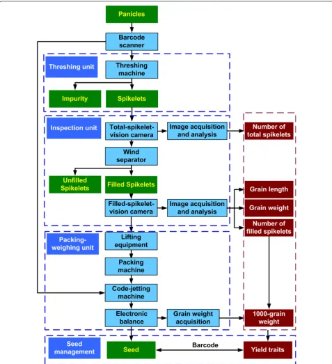
The facility consisted of three major elements: a thresh-ing unit, an inspection unit, and a packthresh-ing-weighthresh-ing unit (Figure 1). The control center used software devel-oped using LabVIEW 8.6 (National Instruments, USA) to control the whole system. The operating procedure includes the following steps: (1) the barcode of the rice plant being evaluated was obtained with a barcode scan-ner or by manual input, depending on the user’s selec-tion. (2) The threshing machine was started as panicles to be processed by the machine were detected. Spikelets were transferred to the inspection unit while impurities were collected at the impurity outlet. (3) The “total-spi-kelet-vision camera” collected images of the total spike-lets (total-spikelet image) that came from the threshing unit (including filled and unfilled spikelets). A wind separator separated the filled spikelets from the unfilled spikelets. The ‘filled-spikelet-vision camera’ collected images of the filled spikelets (filled-spikelet image). The images were analyzed to determine yield traits. Unfilled
spikelets were collected at the unfilled-spikelet outlet. (4) After inspection, lifting equipment raised the col-lected filled spikelets and delivered them to a packing machine for packaging. (5) A code-jetting machine printed the barcode of the recently examined rice plant on the packing bag. (6) An electronic balance weighed the filled spikelets and sent the data to the computer. (7) A collecting device collected the packed filled spike-lets. An additional movie file shows the operation proce-dure in more detail [see Additional file 1].The developed prototype, dubbed the Seed-Evaluation Accelerator (SEA), is shown in Figure 2.
The control flowchart is shown in Figure 3. The times required for panicle feeding (Tf), threshing (Tt),
inspec-tion (Ti), and packing-weighing (Tp) were designed to be
30, 50, 60, and 40seconds, respectively.Tidlewas the idle
time between subsequent measurements and depended on the operator. The threshing unit and the inspection unit worked in parallel with the packing-weighing unit, and Tpwas less than Ti. Thus, the total processing time
per rice plant was determined by Eq. 1:
T=Ti+Tidle (1)
Threshing unit
Panicles were fed into the threshing unit via a panicle inlet. The threshing of the spikelets was triggered by pulses received from a photoelectric sensor attached to the panicle inlet. The machine threshed the spikelets through roller-compaction processes. A sieve was used to separate the spikelets from branches and other unwanted materials. A tilted, vibrating plate under the sieve disaggregated the spikelets as they reached the end of the plate. After the spikelets were vibrated into the spikelet outlet, impurities were blown out through the impurity outlet by an air blower.
Inspection unit
Figure 4 shows the details of the inspection unit. The prototype used two line-scan cameras (Spyder 3 GIGE vision SG-11-02k80-00-R, Teledyne DALSA Company, Germany) to acquire 5000 × 2048 pixel grayscale images with a resolution of 0.23mm/pixel. The cameras were controlled by the computer workstation (HP z600, Hew-lett-Packard Development Company, USA) through an Ethernet card (NI PCIe 8235, National Instruments Cor-poration, USA) that digitized the images into 8-bit files. Two line-array LED light sources served as the illumina-tion system.
the filled spikelets and the unfilled spikelets were sepa-rated by a wind separator mounted between the second and third conveyors. Unfilled spikelets were blown out and collected at an unfilled-spikelet outlet, whereas filled
spikelets fell onto the third conveyor and were imaged by the“filled-spikelet-vision camera”. To spread out the spikelets, the second conveyor was designed with a higher speed than that of the first conveyor, and the
speed of the third conveyor was higher than that of the second. This design produced a separation of individual spikelets and consequently facilitated image analysis. A black conveyor belt was chosen, as it generated good contrast between the belt and spikelets and thus was beneficial for image segmentation.
Packing-weighing unit
As shown in Figure 5, after inspection, the filled spike-lets fell into a grain-collecting tank placed under the third conveyor. Next, lifting equipment raised the tank and poured the filled spikelets into a packing machine. After packing, a code-jetting machine printed the bar-code of the plant being evaluated onto the packing bag. Subsequently, an electronic balance weighed the filled spikelets and sent the grain weight (Wgrain) to the
computer. The TGW was obtained using Eq. 2:
TGW= (Wgrain×1000)
NFS (2)
Communication interface
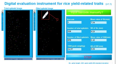
The communication interface is illustrated in Figure 6. The resultant total-spikelet image and the filled-spikelet image, along with the yield trait data, were displayed on the interface. When the“Input barcode manually?” but-ton was clicked, a dialog box was shown to allow users to input the barcode manually.
Automated data and seed management
At the beginning of the yield trait evaluation for each rice plant, the user chose to either scan the barcode of the plant using a barcode scanner or input the barcode manually. This barcode was transferred to the code-jet-ting machine, which then sprayed the barcode on the
Figure 2 The developed prototype of the SEA facility. The facility mainly consisted of three units: a threshing unit for removing spikelets from the panicles, an inspection unit for assessing and measuring yield traits, and a packing-weighing unit for packing and weighing filled spikelets.
Figure 3Control flowchart of the instrument.
packing bag to facilitate seed management. Yield trait data of the rice plant were stored in a Microsoft Excel file along with the barcode of the plant for indexing and data management.
Performance evaluation of the hardware
Rice panicles from 214 harvested Huageng 295 rice plants were tested to evaluate the performance of the prototype. All of the spikelets, including spikelets at the impurity outlet, the unfilled-spikelet outlet and the filled-spikelet outlet (packing machine), were collected. The number of total spikelets and the number of filled
spikelets at the three outlets were counted separately and recorded. For the NTS, NFS and TGW, each rice plant was evaluated three times by different personnel, and the average values were computed as reference data. Manual observations were defined and computed as given in Table 1.
The threshing machine worked well during the tests. The absolute threshing error for total/filled spikelets was calculated as the total/filled spikelet number at the impurity outlet. The percentage threshing error for total/filled spikelets was calculated as the absolute threshing error divided by the number of total/filled spi-kelets of the rice plant being evaluated. Figure 7 ill-ustrates the percentage error of the threshing unit for total spikelets and filled spikelets. As shown in Figure 7, the threshing error for total spikelets was higher than for filled spikelets, indicating that it was more difficult to thresh unfilled spikelets than filled spikelets. It can be observed from Figure 7 that some samples had thresh-ing errors that were significantly higher than the average error. This was because the feeding speed had an impor-tant influence on the threshing of the spikelets. Two panicles entering the threshing machine at the same time would lead to fewer spikelets being threshed. These spikelets that remained on the panicles would be blown out with the panicle branches as impurities and, consequently, increase the threshing error. The mean absolute error and mean absolute percentage error of
Figure 6Software interface of the implemented prototype.
the threshing unit were 34 and 3.33%, respectively, for total spikelets and 19 and 2.27%, respectively, for filled spikelets.
The multi-stage conveyor proved able to segregate most of the spikelets. As a result, most kernels in both the total-spikelet image and the filled-spikelet image were observed to be isolated kernels. The packing-weighing unit worked properly during the test, with average weighing differences of less than 0.01gbetween automatic measurements and manual measurements.
Performance evaluation of the image analysis algorithms
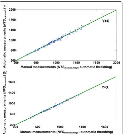
To test the performance of the image analysis algo-rithms, manually threshed spikelets of 90 Huageng 295 rice plants were fed into the inspection unit and imaged by the cameras. Manually threshed spikelets were used to exclude measuring errors caused by threshing. Figure 8 shows the results of manual observation versus image analysis of manually threshed spikelets. In comparison, the image-analysis performance with automatically threshed spikelets coming from the threshing unit was also investigated (Figure 9). The mean absolute error and the mean absolute percentage error with manually threshed spikelets were 22 and 1.36%, respectively, for
the NTS and 7 and 0.54%, respectively, for the NFS. In comparison, the mean absolute error and the mean absolute percentage error with automatically threshed spikelets were 27 and 2.81%, respectively, for the NTS and 15 and 1.77%, respectively, for the NFS. As expected, the measuring accuracy for the manually threshed spikelets was higher than for the automatically threshed spikelets. This was because the threshing machine removed the hulls of some spikelets, and the
Figure 7Performance of the threshing unit. The blue line and red line represent the percentage threshing errors of the threshing unit for total spikelets and filled spikelets, respectively.
Figure 8Performance of the image analysis algorithms with manually threshed spikelets. Scatter plots of manual
measurements versus automatic measurements with manually threshed spikelets for the number of total spikelets and the number of filled spikelets are shown. Ninety Huageng 295 rice plants were used as samples in the evaluation experiment. Least squares linear regression produced the following results: (a) number of total spikelets: line of best fit: y = 1.01x-2.85, correlation coefficient r = 0.9995, (b) number of filled spikelets: line of best fit: y = 0.998x-1.65, correlation coefficient r = 0.9998.
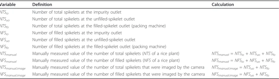
Table 1 Definition and calculation of manual observations
Variable Definition Calculation
NTSio Number of total spikelets at the impurity outlet
NTSuo Number of total spikelets at the unfilled-spikelet outlet
NTSfo Number of total spikelets at the filled-spikelet outlet (packing machine)
NFSio Number of filled spikelets at the impurity outlet
NFSuo Number of filled spikelets at the unfilled-spikelet outlet
NFSfo Number of filled spikelets at the filled-spikelet outlet (packing machine)
NTSmanual Manually measured value of the number of total spikelets (NTSof a rice plant) NTSmanual=NTSio+NTSuo+NTSfo
NFSmanual Manually measured value of the number of filled spikelets (NFSof a rice plant) NFSmanual=NFSio+NFSuo+NFSfo
NTSmanual.image Manually measured value of the number of total spikelets that were imaged by the camera NTSmanual.image=NTSuo+NTSfo
broken hulls would appear in the image as impurities. The external appearance of some broken hulls was simi-lar to a spikelet, and consequently, they would be mista-kenly treated as spikelets. In addition, some brown rice spikelets (spikelets without hulls) were much smaller than normal spikelets and thus would be mistakenly treated as impurities.
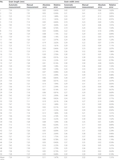
As measuring the GL and the GW of a grain is trou-blesome to perform, the mean GL and GW of only 50 rice plants were measured manually. For each rice plant, 10 filled spikelets were randomly chosen. Five workers measured the grain length and the grain width of each spikelet using a Vernier caliper, and the average value was regarded as the grain length and the grain width of one spikelet. To eliminate measuring errors caused by sampling, the facility measured the same 10 spikelets of each rice plant that were used for the manual measure-ments. The GL and GW of each rice plant were com-puted as the mean grain length and grain width values of the selected 10 spikelets.
Large variances were noted for the GL and GW esti-mation among different personnel. The lack of a
mathematical definition of GL and GW and worker fati-gue under continuous measuring conditions were believed to be two primary reasons for the huge var-iance among workers. Manual measurements and auto-matic measurements for GL and GW are illustrated in Table 2. Generally, automatically measured GL values were slightly larger than the values from manual mea-surements. However, GW values that were measured automatically matched well with those measured manu-ally. The larger GL value from automatic measurement than from manual measurements was because there were errors in the manual location of the maximum length (GL), and inaccurate location of the length invariably leads to underestimation of the GL. Unlike GL measurements, imprecise location of the width may result in underestimation or overestimation of the GW. As a result, the average manually measured GW values matched well with automatically measured values.
Performance evaluation of the whole facility
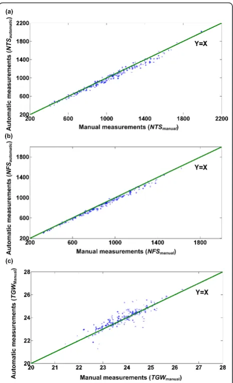
Scatter plots of manual measurements versus automatic measurements of the whole facility for the number of total spikelets, the number of filled spikelets and the 1000-grain weight are shown in Figure 10. As weighing differences between automatic measurements and man-ual measurements were minor, the discrepancy in the TKW between manual and automatic measurements was chiefly caused by NFS measurement differences.
Table 3 summarizes the mean absolute error (MAE, defined by Eq. 3) and the mean absolute percentage error (MAPE, defined by Eq. 4) of the whole facility for the evaluated yield traits. As shown in the table, the facility was capable of evaluating yield traits with mean absolute percentage errors of 4.02%, 3.33%, 1.47%, 1.31% and 1.08% for number of total spikelets, number of filled spikelets, grain length, grain width, and 1000-grain weight, respectively. The MAE and MAPE were com-puted using Eqns. (3) and (4)
MAE = 1 n
n
i=1
|xi.a−xi.m| (3)
MA P E = 1 n
n
i=1
|xi.a−xi.m|
xi.m (4)
where nwas the number of samples, xi.awas the ith
automatically measured value, and xi.m was the ith
manually measured value.
As observed from the results, the measuring error of the NTS was larger than that of the NFS. This was because broken hulls caused by threshing were also imaged by the“total-spikelet-vision camera”. Addition-ally, larger errors can result from broken hulls, which
Table 2 Grain length and grain width measured manually versus automatically (sample size = 50)
No. Grain length (mm) Grain width (mm) Automatic
measurement
Manual measurement
Absolute error
Relative error
Automatic measurement
Manual measurement
Absolute error
Relative error
1 7.34 7.31 0.03 0.46% 3.43 3.37 0.06 1.82%
2 7.32 7.35 0.03 0.36% 3.31 3.41 0.10 2.85%
3 7.23 7.10 0.13 1.88% 3.33 3.21 0.12 3.85%
4 7.43 7.31 0.12 1.65% 3.43 3.27 0.16 4.91%
5 7.19 7.14 0.05 0.66% 3.19 3.23 0.04 1.25%
6 7.45 7.19 0.27 3.69% 3.29 3.23 0.06 1.91%
7 7.31 7.26 0.06 0.76% 3.19 3.24 0.05 1.54%
8 7.12 7.09 0.03 0.38% 3.22 3.32 0.10 2.94%
9 7.38 7.29 0.08 1.14% 3.32 3.29 0.03 0.84%
10 7.39 7.31 0.08 1.14% 3.30 3.33 0.03 0.81%
11 7.41 7.20 0.21 2.97% 3.24 3.28 0.04 1.23%
12 7.40 7.21 0.19 2.62% 3.29 3.22 0.07 2.15%
13 7.25 7.13 0.12 1.61% 3.29 3.33 0.04 1.11%
14 7.16 7.13 0.03 0.46% 3.29 3.23 0.07 2.07%
15 7.39 7.23 0.15 2.14% 3.26 3.32 0.06 1.86%
16 7.51 7.31 0.20 2.76% 3.28 3.33 0.05 1.39%
17 7.19 7.13 0.06 0.91% 3.26 3.28 0.02 0.52%
18 7.46 7.29 0.16 2.25% 3.37 3.40 0.03 0.79%
19 7.27 7.28 0.01 0.14% 3.30 3.30 0.00 0.02%
20 7.29 7.20 0.09 1.28% 3.32 3.36 0.04 1.33%
21 7.32 7.23 0.09 1.29% 3.24 3.33 0.09 2.57%
22 7.33 7.25 0.07 0.98% 3.29 3.36 0.07 2.15%
23 7.52 7.37 0.15 2.09% 3.24 3.39 0.15 4.48%
24 7.38 7.32 0.06 0.85% 3.28 3.37 0.08 2.48%
25 7.33 7.33 0.00 0.01% 3.32 3.43 0.11 3.07%
26 7.36 7.22 0.14 1.94% 3.29 3.31 0.02 0.65%
27 7.36 7.19 0.17 2.39% 3.33 3.29 0.04 1.09%
28 7.28 7.29 0.01 0.14% 3.31 3.29 0.02 0.67%
29 7.24 7.18 0.06 0.81% 3.27 3.29 0.02 0.60%
30 7.42 7.28 0.15 2.00% 3.48 3.41 0.07 2.05%
31 7.33 7.27 0.06 0.82% 3.24 3.33 0.09 2.71%
32 7.29 7.11 0.19 2.61% 3.36 3.27 0.10 2.94%
33 7.47 7.35 0.12 1.68% 3.31 3.31 0.00 0.03%
34 7.26 7.24 0.02 0.21% 3.41 3.41 0.00 0.00%
35 7.59 7.42 0.17 2.22% 3.42 3.39 0.03 0.92%
36 7.31 7.18 0.13 1.80% 3.26 3.21 0.05 1.41%
37 7.36 7.20 0.16 2.16% 3.35 3.33 0.02 0.47%
38 7.50 7.26 0.23 3.22% 3.34 3.30 0.05 1.42%
39 7.36 7.28 0.08 1.09% 3.36 3.35 0.01 0.28%
40 7.12 7.13 0.02 0.26% 3.14 3.17 0.03 0.80%
41 7.34 7.15 0.19 2.67% 3.32 3.31 0.01 0.24%
42 7.21 7.26 0.05 0.69% 3.24 3.31 0.08 2.29%
43 7.39 7.20 0.19 2.64% 3.36 3.38 0.02 0.46%
44 7.37 7.24 0.13 1.75% 3.35 3.37 0.02 0.48%
45 7.38 7.32 0.06 0.78% 3.32 3.38 0.06 1.74%
46 7.24 7.20 0.03 0.46% 3.37 3.35 0.02 0.59%
47 7.42 7.26 0.16 2.23% 3.30 3.34 0.05 1.41%
48 7.59 7.39 0.21 2.79% 3.35 3.36 0.01 0.21%
49 7.38 7.32 0.05 0.73% 3.37 3.39 0.02 0.63%
50 7.28 7.23 0.05 0.68% 3.30 3.30 0.00 0.10%
Mean value
are very similar in appearance to complete spikelets and, consequently, may be treated as spikelets by the vision system but are ignored in manual observation. These broken hulls were blown out into the impurity outlet by the wind separator and thus would not influ-ence the NFS measurement. Anther reason for the lar-ger measuring error of the NTS was that the threshing error of the total spikelets was larger than that of the filled spikelets.
The threshing error directly decreases the number of spikelets that pass through the inspection unit and, consequently, influences the measuring accuracy of the NTS and the NFS. The relation between the threshing error and the measuring error of the NTS and the NFS were investigated. Figure 11 shows the variation of the percentage measuring error of the facility for the NTS and the NFS as a percentage threshing error changes. As shown in Figure 11, the measuring error for both the NTS and the NFS pre-sented an upward trend as the threshing error increased. Compared with the measuring error for the NFS, the measuring error for the NTS had a weaker relationship with the threshing error. This was because broken hulls had a considerable effect on the NTS measuring error.
Figure 10 Performance of the entire facility. Scatter plots of manual measurements versus automatic measurements with the facility for (a) the number of total spikelets, (b) the number of filled spikelets, and (c) the 1000-grain weight are shown. In total, 214 Huageng 295 rice plants were used as samples in the evaluation experiment. Least squares linear regression produced the following results: (a) number of total spikelets: line of best fit: y = 0.96x+10.24, correlation coefficient r = 0.992, (b) number of filled spikelets: line of best fit: y = 0.96x+6.14, correlation coefficient r = 0.996, (c) 1000-grain weight: line of best fit: y = 0.94x+1.56, correlation coefficient r = 0.91.
Table 3 Mean absolute error (MAE) and mean absolute percentage error (MAPE) for the evaluated traits (asample size = 214,bsample size = 50)
Trait Definition MAE MAPE
NTSa Number of total spikelets of a rice plant 41 4.02%
NFSa Number of filled spikelets of a rice plant 29 3.33%
GLb Average grain length of a rice plant 0.11mm 1.47%
GWb Average grain width of a rice plant 0.04mm 1.31%
TGWa 1000-grain weight of a rice plant 0.26g 1.08%
Measuring the efficiency of the whole facility
Assuming Tidle was 0 s, the total processing time per
rice plant was approximately 60 s (calculated as Eq. 1); i.e., the implemented prototype was able to perform yield trait evaluations for approximately 1440 rice plants per 24 h continuous workday. Generally, an experienced worker can evaluate approximately 20 plants per day (working 8 hours per day). As the prototype needs no human operation except for panicle feeding, it is feasible to run the facility continuously for 24 hours for mass measurements. From this point of view, the facility was capable of evaluating rice yield traits with an efficiency more than 70 times greater than that of manual opera-tion at its maximum throughput.
The efficiency of the whole facility was determined by the inspection unit and the time elapsed, which was lim-ited by the threshing time. More effective threshing methods will be developed in the future to improve the efficiency of the whole facility. The software was designed to allow the images to be processed concur-rently as the cameras were acquiring images. Image pro-cessing requires less time than image acquisition. The shorter time needed for image processing also opened up the possibility of applying more sophisticated algo-rithms for more sophisticated solutions. For instance, statistical classifiers such as the distance classifier, discri-minant analysis and artificial neural networks could be adapted in the future to discriminate broken hulls from spikelets.
Automation and integration of threshing, multi-trait measurement and seed packing
With the only manual operation being panicle feeding, the SEA facility automated the entire process of thresh-ing, fast multi-trait measurement and seed packing. The yield traits were automatically observed and stored with a unique code after system inspection. Meanwhile, the seeds were automatically packed with the relevant code. The automation and integration of the entire process will substantially improve the yield trait evaluation pro-cess for rice researchers. With the data tracking ability, it was convenient for the user to manage and analyze data. Data tracking also allowed the user to combine yield traits with other traits such as the tiller number, the leaf area, the plant height, thus allowing an inte-grated understanding. Moreover, data tracking is benefi-cial for seed management. Compared with manual data logging and seed management, the data tracking of the facility made data management and seed management more robust and reliable.
Conclusions
This paper described an engineering prototype for the automatic evaluation of rice yield traits, including the
number of total spikelets, the number of filled spikelets, the grain length, the grain width, and the 1000-grain weight. The prototype comprised three major units: the threshing unit, the inspection unit, and the packing-weighing unit. The mean absolute percentage error was less than 5% for all of the evaluated yield traits, and the efficiency was approximately 1440 plants per 24-hours continuous workday. The facility will be helpful for improving the accuracy and efficiency of rice yield trait evaluation and will serve as a powerful tool in rice plant phenotyping, which will eventually benefit rice breeding, genetic research, functional genomics research and other rice research. With some modifications, the appli-cation could be extended and generalized to other crops, such as wheat, corn and barley. Other compound yield traits such as the seed setting rate and the length-width ratio can also be deduced from the extracted traits. In summary, using agricultural photonics, the high-throughput facility, dubbed the Seed-Evaluation Accelerator, gives plant scientists a novel tool to unlock the phenotypic information coded in rice genome [25].
Methods
Image acquisition
The control software was designed for evaluating yield traits of one rice plant at a time. The continuous acqui-sition of the images was controlled by the pulses received from a photoelectric sensor attached to the panicle inlet of the threshing unit. Images were acquired and stored using the NI-IMAQ Virtual Instruments (VI) Library for LabVIEW (National Instruments Corpora-tion, USA). For each plant, 14 images were acquired by the“total-spikelet-vision camera”(called the total-spike-let image) and 20 images were acquired by the “filled-spikelet-vision camera”(called the filled-spikelet image). This design was applicable to most rice varieties with less than 20 panicles per plant. Figure 12 shows typical total-spikelet and filled-spikelet images acquired by the two cameras. Note that the images shown in Figure 12 have been cropped for better visualization, as the origi-nal images are too large (5000 × 2048 pixels).
Image analysis
The image-analysis software was programmed using NI Vision for LabVIEW 8.6 (National Instruments Corpora-tion, USA). The software was designed to allow the two cameras (the “total-spikelet-vision camera” and the “filled-spikelet-vision camera”) to work at the same time, and the images were analyzed in the computer simultaneously while the cameras were acquiring new images, thus optimizing the measurement efficiency.
segmentation was performed to determine the back-ground and objects of interest. For better processing speed, a pixel-oriented segmentation algorithm was applied in this study. A pixel was considered to belong to a background point if its grayscale fell below a pre-defined, fixed threshold. In a subsequent step, a median filter (3 × 3 neighborhood) was used to remove isolated pixels. As some small pieces of branches may appear on the conveyor, objects with a length-width ratio greater than three times that of the spikelets were treated as branches and removed. Branches with a length-width ratio less than three times that of the spikelets were
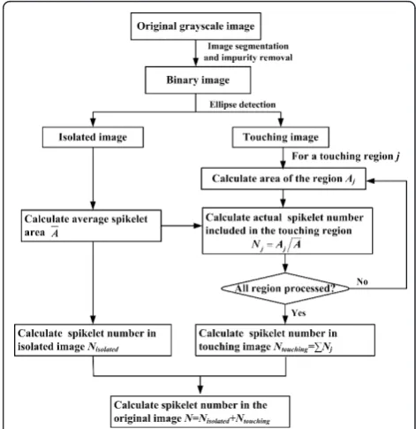
subsequently removed using the “IMAQ detect line” operation. Small regions with an area less than half of the average area of spikelets were regarded as impurities and removed from the image. Spikelets may be touching during on-line processing. The shape of an isolated spi-kelet is roughly elliptical, so the“IMAQ detect Ellipse” operation was used to identify the isolated spikelet in the image (NI Vision Concepts Manual, National Instru-ments Corporation, USA). After identification, the origi-nal image was divided into two images, one image with only the isolated spikelet (isolated image) and the other with only the touching spikelets (touching image). From an efficiency perspective, we opted for a simple area-determination method to determine the spikelet number in the touching imageNtouching, which was computed by
Eq. 5 and Eq. 6:
Nj= round (Aj
A) (5)
Ntouching= T
j=1
Nj (6)
where Njwas the actual spikelet number for a given
touching region jin the touching image, the function round(x) rounded x to the nearest integer,Aj was the
area of the touching regionj,Ā was the average spikelet area calculated from the isolated image, andT was the number of touching regions.
The spikelet number (N) in the original image was determined by summing up the spikelet numbers in the
Figure 12 Typical grayscale images for (a) a total-spikelet image and (b) a filled- spikelet image.
isolated image (Nisolated) and in the touching image
(Ntouching). The NTS of the evaluated plant was
calcu-lated as the sum of the spikelet numbers in all 14 total-spikelet images. Similarly, the NFS of the evaluated plant was calculated as the sum of the spikelet numbers in all 20 filled-spikelet images.
The length and width of each isolated spikelet in the filled-spikelet images were calculated. The GL is defined as the maximum Euclidean distance between two boundary points of a filled spikelet, and the GW is defined as the maximum length of straight lines perpen-dicular to the line of the GL.
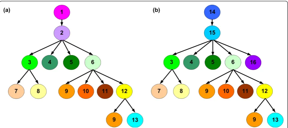
Figure 14 shows the structure of the image-processing program in LabVIEW for total-spikelet images and filled-spikelet images. Illustrations showing block dia-grams of the VIs developed in this research are attached in Additional files 2, 3, 4, 5, 6, 7, 8, 9, 10, 11, 12, 13, 14, 15, 16, and 17.
Additional material
Additional file 1: Operating procedure of the facility. A video showing the detailed operating procedure of the SEA facility.
Additional file 2: Source code file 1.
ImProcessPerPlant_TotalSpikeletImage.vi was used for processing total-spikelet images of one plant (14 images in the developed facility). The number of total spikelets of the evaluated plant was calculated as the sum of the spikelet numbers in all 14 total-spikelet images. Note that in
the facility, ImProcessPerPlant_TotalSpikeletImage.vi functions were included in a‘queue’structure to allow images to be analyzed in the computer simultaneously while the cameras were acquiring new images, thus optimizing the measuring efficiency.
Additional file 3: Source code file 2. ImageAnalysis_TotalSpikeletImage. vi was developed for processing a single total-spikelet image.
Additional file 4: Source code file 3. ImagePreProcess.vi executed image segmentation and impurity removal.
Additional file 5: Source code file 4. In continuous image acquisition, some grains may exist both in the bottom border of the previous image and in the top border of the subsequent image. Merge.vi. merged the object at the bottom border of the previous image with the other part of the object in the subsequent image.
Additional file 6: Source code file 5. Split.vi extracted objects at the bottom border in the current image.
Additional file 7: Source code file 6. ImageProcess.vi removed small particles and calculated spikelet number in an image.
Additional file 8: Source code file 7. ImpurityRemove.vi removed objects with a length-width ratio greater than three times that of the spikelets.
Additional file 9: Source code file 8. StemRemove.vi removed branches with length-width ratios less than three times that of the spikelet using the“IMAQ detect line”operation.
Additional file 10: Source code file 9. MeanAreaCalculation.vi calculated the average area of the spikelets.
Additional file 11: Source code file 10. RemoveSmallParticle.vi removed small regions with an area less than the defined area threshold.
Additional file 12: Source code file 11. GrainClassification.vi divided the original image into two images: one image with only isolated spikelets (isolated image) and the other with only touching spikelets (touching image).
Figure 14Structure of image processing program in LabVIEW for (a) total-spikelet images and (b) filled-spikelet images. 1: Source code file 1 (ImProcessPerPlant_TotalSpikeletImage.vi), 2: Source code file 2 (ImageAnalysis_TotalSpikeletImage.vi), 3: Source code file 3
(ImagePreProcess.vi), 4: Source code file 4 (Merge.vi), 5: Source code file 5(Split.vi), 6: Source code file 6 (ImageProcess.vi), 7: Source code file 7 (ImpurityRemove.vi), 8: Source code file 8 (StemRemove.vi), 9: Source code file 9 (MeanAreaCalculation.vi), 10: Source code file 10
(RemoveSmallParticle.vi), 11: Source code file 11 (GrainClassification.vi), 12: Source code file 12 (TotalGrainNumberCalculation.vi), 13: Source code file 13 (TouchingGrainNumberCalculation.vi), 14: Source code file 14 (ImProcessPerPlant_FilledSpikeletImage.vi), 15: Source code file 15
Additional file 13: Source code file 12. TotalGrainNumberCalculation.vi determined the spikelet number in the original image by summing up the spikelet number in the isolated image and the spikelet number in the touching image.
Additional file 14: Source code file 13.
TouchingGrainNumberCalculation.vi calculated the spikelet number in the touching image.
Additional file 15: Source code file 14.
ImProcessPerPlant_FilledSpikeletImage.vi was used for processing filled-spikelet images of one plant (20 images in the developed facility). The number of filled spikelets of the evaluated plant was calculated as the sum of the spikelet numbers in all 20 filled-spikelet images. Note that in on-line measurements, ImProcessPerPlant_FilledSpikeletImage.vi functions were included in a‘queue’structure to allow images to be analyzed in the computer simultaneously while the cameras were acquiring new images.
Additional file 16: Source code file 15.
ImageAnalysis_FilledSpikeletImage.vi was developed for processing a single filled-spikelet image.
Additional file 17: Source code file 16. GetLengthWidthRatio.vi calculated the length, width, and length-width ratio for each isolated grain.
Acknowledgements
The authors deeply appreciate the cooperation of our partners at Huazhong Agricultural University for providing the grain samples. This work was supported the Key Program of the Natural Science Foundation of Hubei Province (Grant No. 2008CDA087) and the Program for New Century Excellent Talents in University (No. NCET-10-0386).
Author details
1Britton Chance Center for Biomedical Photonics, Wuhan National Laboratory
for Optoelectronics-Huazhong University of Science and Technology, 1037 Luoyu Rd., Wuhan 430074, P.R. China.2Key Laboratory of Biomedical
Photonics of Ministry of Education, College of Life Science and Technology, Huazhong University of Science and Technology, 1037 Luoyu Rd., Wuhan 430074, P.R. China.
Authors’contributions
LD developed the software, performed the evaluation experiment, analyzed the data, and drafted the manuscript. WY designed and built the hardware, performed the evaluation experiment, and contributed in writing the manuscript. CH provided support with hardware development and implementation of the evaluation experiment. QL supervised the study and contributed in writing the manuscript. All of the authors read and approved the final manuscript.
Competing interests
The authors declare that they have no competing interests.
Received: 18 October 2011 Accepted: 12 December 2011 Published: 12 December 2011
References
1. Zhang Q:Strategies for developing green super rice.PNAS2007,
104(42):16402-16409.
2. Wang E, Wang J, Zhu X, Hao W, Wang L, Li Q, Zhang L, He W, Lu B, Lin H, Ma H, Zhang G, He Z:Control of rice grain-filling and yield by a gene with a potential signature of domestication.Nature Genetics2008,
40(11):1370-1374.
3. Xing Y, Zhang Q:Genetic and molecular bases of rice yield.Annual Review of Plant Biology2010,61:11.1-11.22.
4. Prasertsak A, Fukai S:Nitrogen availability and water stress interaction on rice growth and yield.Field Crops Research1997,52:249-260.
5. Xiao J, Li J, Grandillo S, Ahn SN, Yuan L, Tanksley SD, McCouch SR:
Identification of trait-improving quantitative trait loci alleles from a wild rice relative, Oryza rufipogon.Genetics1998,150:899-909.
6. Thomson MJ, Tai TH, McClung AM, Lai XH, Hinga ME, Lobos KB, Xu Y, Martinez CP, McCouch SR:Mapping quantitative trait loci for yield, yield components and morphological traits in an advanced backcross population between Oryza rufipogon and the Oryza sativa cultivar Jefferson.Theoretical and Applied Genetics2003,107:479-493. 7. Bagge M, Lübberstedt T:Functional markers in wheat: technical and
economic aspects.Molocular Breeding2008,22:319-328.
8. Kolukisaoglu Ü, Thurow K:Future and frontiers of automated screening in plant sciences.Plant Science2010,178:476-484.
9. Bylesjö M, Segura V, Soolanayakanahally RY, Rae AM, Trygg J, Gustafsson P, Jansson S, Street NR:LAMINA: a tool for rapid quantification of leaf size and shape parameters.BMC Plant Biology2008,8:82-90.
10. French A, Ubeda-Tomás S, Holman TJ, Bennett MJ, Pridmore T: High-throughput quantification of root growth using a novel image-analysis tool.Plant physiology2009,150:1784-1795.
11. Yazdanbakhsh N, Fisahn J:High throughput phenotyping of root growth dynamics, lateral root formation, root architecture and root hair development enabled by PlaRoM.Functional Plant Biology2009,
36:938-946.
12. Wang L, Uilecan IV, Assadi AH, Kozmik CA, Spalding EP:HYPOTrace: image analysis software for measuring hypocotyl growth and shape demonstrated on Arabidopsis seedlings undergoing photomorphogenesis.Plant physiology2009,149:1632-1637. 13. Yang W, Xu X, Duan L, Luo Q, Chen S, Zeng S, Liu Q:High-throughput
measurement of rice tillers using a conveyor equipped with X-ray computed tomography.Review of Scientific Instruments2011,
82(2):025102-025109.
14. Golzarian MR, Frick RA, Rajendran K, Berger B, Roy S, Tester M, Lun DS:
Accurate inference of shoot biomass from high-throughput images of cereal plants.Plant Methods2011,7:2.
15. Granier C, Aguirrezabal L, Chenu K, Cookson SJ, Dauzat M, Hamard P, Thioux JJ, Rolland G, Bouchier-Combaud S, Lebaudy A, Muller B, Simonneau T, Tardieu F:PHENOPSIS, an automated platform for reproducible phenotyping of plant responses to soil water deficit in Arabidopsis thaliana permitted the identification of an accession with low sensitivity to soil water deficit.New Phytologist2006,169:623-635. 16. Reuzeau C, Pen J, Frankard V, Wolf J, Peerbolte R, Broekaert W, Camp W:
TraitMill: a discovery engine for identifying yield-enhancement genes in Cereals.Molecular Plant Breeding2005,3(5):753-759.
17. The Plant Accelerator.[http://www.plantaccelerator.org.au/]. 18. The High Resolution Plan Phenotyping Centre.[http://www.
plantphenomics.org.au/HRPPC].
19. The Leibniz Institute of Plant Genetics and Crop Plant Research (IPK).
[http://www.ipk-gatersleben.de].
20. Institute of Biological, Environmental and Rural Sciences (IBERS).[http:// www.aber.ac.uk/en/ibers/].
21. French National Institute for Agricultural Research (INRA).[http://www. international.inra.fr/].
22. Duan L, Yang W, Bi K, Chen S, Luo Q, Liu Q:Fast discrimination and counting of filled/unfilled rice spikelets based on bi-modal imaging.
Computers and Electronics in Agriculture2011,75:196-203. 23. Igathinathane C, Pordesimo LO, Batchelor WD:Major orthogonal
dimensions measurement of food grains by machine vision using ImageJ.Food Research International2009,42:76-84.
24. Igathinathane C, Pordesimo LO, Columbus EP, Batchelor WD, Methuku SR:
Shape identification and particles size distribution from basic shape parameters using ImageJ.Computers and Electronics In Agriculture2008,
63:168-182.
25. Finkel E:With‘Phenomics,’plant scientists hope to shift breeding into overdrive.Science2009,325:380-381.
doi:10.1186/1746-4811-7-44
Cite this article as:Duanet al.:A novel machine-vision-based facility for the automatic evaluation of yield-related traits in rice.Plant Methods