Vol 4, No. 1, (2014), pp 41-56
A numerical technique based on
operational matrices for solving
nonlinear integro-differential equations
A. Golbabai
Abstract
This paper presents a computational method for solving two types of integro-differential equations, system of nonlinear high order Volterra-Fredholm differential equation(VFIDEs) and nonlinear fractional order integro-differential equations. Our tools for this aims is operational matrices of inte-gration and fractional inteinte-gration. By this method the given problems reduce to solve a system of algebraic equations. Illustrative examples are included to demonstrate the efficiency and high accuracy of the method.
Keywords: Operational matrix of integration; Volterra-Fredholm; Non-linear system of integro-differential equations; Fractional order; Legendre wavelet.
1 Introduction
Integro-differential equations frequently appear in all fields of sciences such as physics, chemistry and engineering problems [11, 20, 23, 24]. In last few decades fractional calculus and fractional differential equations have found application in several different disciplines, many important phenomena in electromagnetic, acoustics, viscolasticity, electrochemistry and material sci-ence are well described by differentiable and integro differentiable equation of fractional order[3, 22]. There are various numerical and analytical meth-ods to solve such problems, for example, the homotopy perturbation method [4, 7, 8, 9], the Adomian decomposition method [5], fractional differential transform method [21] and Gronwald–Letnikov discretization method [6].
In recent years the approximation of orthogonal functions has been play-ing role in the solution of different kinds of mathematical and engineerplay-ing problems such as identification, analysis and optimal control[15, 16, 18]. The main feature of this technique is to reduce the integro-differential equations
Received 9 September 2013; revised 11 December 2013; accepted 8 January 2014 A. Golbabai
Islamic Azad university, Karaj Branch, Karaj, Iran. e-mail: [email protected]
to a nonlinear algebraic equation by introducing integration matrix of basis functions. In present article, we are concerned with the application of Leg-endre wavelet to the numerical solution of:
(I). Nonlinear fractional order integro-differential equations
D∗αtu(t) =f(t) +
∫ x
0
K(t, u(t), D∗αtu(t))dt, 0≤α <1. (1)
(II). Nonlinear system of high order (VFIDe) of the form
n
∑
j=0
pij(x)ul
(j)
(x) =fi(x) +λi1 ∫x
0 Ki1(x, t, u(t), u′(t), . . . , u
(n)(t))dt +λi2
∫1
0 Ki2(x, t, u(t), u′(t), . . . , u
(n)(t))dt, i= 1, . . . , s, (2) whereu(j)(x) =(u(j)
1 , . . . , u (j)
s
)
forj= 0, . . . , n and initial conditions are
u(ij)(0) =aj, j= 0,1. . . , n−1, (3)
where f(x),K, Ki1 and Ki2 are known functions assumed to be in L2(R) on the interval 0 ≤x, t≤1, u(t) is unknown, Ki1 and Ki2 are nonlinear in x, t, u(t), . . . , u(n)(t). This type of equations whose integrand contain high order derivatives arise in many fields such as theory of elasticity .
The article is organized as follows: in Section 2 we define the Legendre wavelets and operational matrix of integration. Section 3 is devoted to the solution of Eq. (1). In Section 4, we obtain an error bound for our method. Section 5, include our numerical findings and demonstrate the accuracy of the proposed scheme.
2 Preliminaries and notation
This section gives some necessary definition and mathematical preliminaries of the fractional calculus theory which are used further in this paper. The Riemann-Lioville fractional integration of orderα >0 is defined as [14]
Itαf(t) = Γ(1α) ∫t
0
f(τ) (t−τ)(1−α)dτ, It0f(t) =f(τ),
(4)
and its fractional derivative of order α >0 is normally used:
Dtαf(t) = (
d dt)
n
Itn−αf(t) (n−1< α≤n), (5)
Itαtυ= Γ(υ+ 1) Γ(α+υ+ 1)t
υ+α. (6)
The modified fractional differential operatorD∗αt proposed by Caputo is
Dα∗tf(t) =
1 Γ(n−α)
∫t
0(t−τ)
n−α−1
f(n)(τ) (n−1< α≤n),
dn
dtnf(t) α=n∈N,
(7)
wherenis an integer. Caputos integral operator has an useful property:
ItαDα∗tf(t) =f(t)−
n∑−1
k=0
f(k)(0+)t
k
k!, (n−1< α≤n), (8)
wherenis an integer.
3 Properties of Legendre wavelet
3.1 Wavelets and Legendre wavelet
Wavelet constitute a family of functions constructed by a single function called the mother wavelet. When the dilation parameter a and translation parameter b vary continuously, we have the following family of continuous wavelet as [10]
ψ(a,b)=|a|− 1/2
ψ(t−b
a ), a, b∈R, a̸= 0.
If we restrict the parameters a and b to discrete values as a = a−0m, b =
kb0a−0m, a0>1, b0>0 andm, k∈Z.We have the following family of discrete wavelets
ψm.k(t) =|a0|
m/2
ψ(am0t−kb0),
where ψm.k(t) forms a wavelet basis for L2(R). In particular, whena0 = 2, b0= 1, ψm.k(t) forms an orthonormal basis.
The Legendre wavelets are defined on interval [0,1) see [16, 17].
ψnm=
√
m+122k/2L
m(2kt−ˆn), f ornˆ2−k1 ≤t < ˆ
n+1 2k ,
0 otherwise,
of order m which are defined on the interval [- 1,1] and can be determined with the aid of the following recurrence formulae:
L0(t) = 1, L1(t) =t,
Lm+1(t) = ( 2m+ 1
m+ 1 )tLm(t)−(
m
m+ 1)Lm−1(t), m= 1,2,3, . . .
3.2 Function approximation
Theorem.A functionf(t)defined on [0,1) can be expanded as infinite sum of Legendre wavelets, and the series converges uniformly to the functionf(x), that is
f(t) = ∞ ∑
n=1 ∞ ∑
m=0
cnmψnm(t), (9)
where, cnm= (f(t), ψnm(t)), in which(., .)denote the inner product.
Proof.see[13].
If the infinite series in Eq. (9) is truncated, then it can be written as
f(t)≃ 2k−1
∑
n=1
M∑−1
m=1
cnmψnm(t) =CTΨ(t), (10)
whereC and Ψ(t) are 2M ×1 matrices given by
C= [c10, c11, . . . , c1M−1, c20, . . . , c2M−1, . . . , c2k−10, . . . , c2k−1M]
T
, (11)
Ψ(t) = [ψ10, ψ11, . . . , ψ1M−1, ψ20, . . . , ψ2M−1, . . . , ψ2k−10, . . . , ψ2k−1M]T.
(12) Now we want to find an upper bound to the estimate error . Suppose that
f(x) is a (m+ 1)−times differentiable function on Ω = [0,1). An error function between f(x) and its Legendre-wavelet approximation fnm(x) is
defined on every subinterval Ωn= [nˆ2−k1 ≤t < ˆ
n+1 2k ] as
enm(x) =f(x)−fnm(x) =f(x)−cnmψnm(x). (13)
Then we can write
∥enm(x)∥
2 =
∫ nˆ+1 2k
ˆ
n−1 2k
|f(x)−cnmψnm(x)|
2
. (14)
Since ψnm(x) is a polynomial of degree m,we can use the error bound for
|f(x)−pn(x)| ≤
h(m+1)
4(m+ 1)ξ∈[nˆmax−1 2k ,
ˆ
n+1 2k ]
f(m+1)(ξ), (15)
whereh= 1
2km.By Eq. (14)and Eq. (15) ∥enm(x)∥
2≤∫nˆ2+1k
ˆ
n−1 2k
h
(m+1)
4(m+1) max
ξ∈[nˆ−1
2k ,
ˆ
n+1 2k ]
f(m+1)(ξ) 2 ≤ 1 2k h
(m+1)
4(m+1) max
ξ∈[nˆ−1 2k ,
ˆ
n+1 2k ]
f(m+1)(ξ)
2 . (16)
According to above equation we find an error bound for each subinterval as
∥enm(x)∥ ≤
1 2k/2
h(m+1)
4(m+ 1)ξ∈[nˆmax−1 2k ,
ˆ
n+1 2k ]
f(m+1)(ξ). (17)
Then for error on Ω we get
∥e(x)∥ ≤ 1 2k/2
h(m+1) 4(m+ 1)ξmax∈[0,1]
f(m+1)(ξ). (18)
3.3 The Legendre wavelets operational matrix of
integration
The integration of the Vector defined in Eq.(12) can be obtained as ∫ t
0
Ψ(t′)dt′=PΨ(t), (19)
whereP is the 2k−1M×2k−1M operational matrix for integration [18]
P= 1 2k
L H H H · · · H
0 L H H · · · H
0 0 L H · · · H
..
. ... ... . .. . .. · · · 0 0 0 · · · L H
0 0 0 0 · · · L
.
H =
2 0 · · · 0 0 0 · · · 0
· · · · . .. ... 0 0 · · · 0
,
and
L=
1 311/2 0 0 · · · 0 0 0
−31/2
3 0
31/2
3×51/2 0 · · · 0 0 0
0 − 51/2 5×31/2 0
51/2
5×71/2 0 0 0
0 0 − 71/2
7×51/2 0 . .. 0 0 0
..
. ... ... ... . .. . .. . .. ...
0 0 0 0 · · · −(2M(2M−3)(2M−3)1−/25)1/2 0
(2M−3)1/2 (2M−3)(2M−1)1/2
0 0 0 0 · · · 0 −(2M(2M−1)(2M−1)1−/23)1/2 0
.
3.4 Operational matrix of fractional integration
We defined am-set of Block Pulse function (BPF)as:
bi(t) =
{
1, i/m≤t <(i+ 1)/m
0, otherwise, (20)
wherei= 0,1,2, . . .(m−1).
The functionbi(t) are disjoint and orthogonal. That is
bi(t)bj(t) =
{
0, i̸=j bi(t), i=l.
(21)
The Legendre wavelet may be expanded into m-terms of block pulse function (BPF) as
Ψm(t) = Φm×mBm(t), (22)
where
Bm(t)
∆
= [b0(t)b1(t). . . bi(t). . . b(m−1)(t) ]T. (23) The Block Pulse operational matrix of the fractional integration give in [12]
Fαas following:
(ItαBm)(t)≈FαBm(t), (24)
Fα= 1
mα
1 Γ(α+ 2)
1ξ1ξ2 · · · ξ(m−1) 0 1 ξ1 · · · ξ(m−2) 0 0 1 · · · ξ(m−3) 0 0 0 . .. ...
0 0 0 0 1
.
withξk= (k+ 1)α+1−2kα+1+ (k−1)α+1. The Legendre wavelet operational
matrix of of fractional integration is defined in [19] as
Pmα×m= Φm×mFαΦ−m1×m, (25)
so the fractional integration of vector in Eq. (12) is defined as
(ItαΨ)(t)≈PαΨm(t). (26)
4 Application to nonlinear system of VFIDEs
Here, before presenting our method, we prove the next lemma. By this lemma we can approximate the high order derivative of a function by Legen-dre wavelet.
Lemma. Suppose that u(x) = CTΨ(x) where C and Ψ(x) are defined in Eq. (11) and Eq. (12), then
u(k)(x) = (CTP−k−
k−1 ∑
i=0
u(0i)ETPi−k)Ψ(x), (27)
where P is operational matrix of integration,u(i)(0) =u(i)
0 andE is defined asETΨ(t) = 1.
Proof. suppose that f(x) = uk(x) and we approximate u(x) and f(x) by
Legender wavelet as {
u(x) =CTΨ(x),
f(x) =FTΨ(x), (28)
by integratingf(t) on [0, t] ∫t
0 ∫t
0. . . ∫t
0f(t′)dt| {z }′. . . dt′
k−times
=∫0t∫0t. . .∫0tFTPΨ(t′)dt′. . . dt′
| {z } (k−1)times
=∫0t∫0t. . .∫0tFTP2Ψ(t′)dt′. . . dt′ | {z } (k−2)times
.. .
=FTPkΨ(t),
Sincef(x) =uk(x), then
∫t
0 ∫t
0· · · ∫t
0f(t′)dt| {z }′· · ·dt′
k−times
=∫0t∫0t· · ·∫0t(u(k−1)(t)−u(k−1)(0))d(t′)· · ·dt′
| {z }
(k−1)−times
=∫0t∫0t· · ·∫0tu(k−1)(t) dt′· · ·dt′ | {z } (k−1)−times
u(k−1)(0)∫t 0
∫t
0· · · ∫t
0 dt ′· · ·dt′ | {z } (k−1)−times
.. .
=u(t)−u(0)(0)−u(1)(0)− · · · −u(k−1)(0)∫t 0
∫t
0· · · ∫t
0 dt| {z }′· · ·dt′ (k−1)−times
,
(30) byu(i)(0) =u(0i) we get
u(0i)
∫ t
0 ∫ t
0 · · ·
∫ t
0
dt′· · ·dt′
| {z }
k−times
=u(0i)ETPiΨ(t), (31)
Eq. (29)-(31) result
FTPkΨ(t) =CΨ(t)−u(0)
0 ETΨ(t)−u (1)
0 ETPΨ(t)− · · · −u (k−1)
0 ETPk−1Ψ(t) =CTΨ(t)−k∑−1
i=0
u(0i)ETPiΨ(t),
(32) Since the basis functions are linear independent, we omit Ψ(t) from both sides of Eq. (32), then this equation can be written as
FTPk =CT −
k−1 ∑
i=0
u(0i)ETPi, (33) and then
FT =CTP−k−
k−1 ∑
i=0
u(0i)ETPi−k, (34) according to Eq. (28)
u(k)(x) = (CTP−k−
k−1 ∑
i=0
u(0i)ETPi−k)Ψ(x). (35) This ends the proof of lemma. □
To solve Eq. (2) by Legendre wavelets, we assume that eachuℓ(x) has the
expansion as
uℓ(x) =CℓTΨ(x), ℓ= 1, . . . , s, (36)
yℓ(k)(x) = (CℓTP−k−
k−1 ∑
i=0
y(ℓi0)ETPi−k)Ψ(x), ℓ= 1, . . . , s, (37) substituting Eq. (36) and Eq. (37) in Eq. (2) results forℓ= 1, . . . , s
pℓ0CℓTΨ(x) + n
∑
i=1
pℓi(x)(CℓTP− i− i∑−1
m=0
u(ℓm0)ETPm−i)Ψ(x) =f ℓ(x)
+λℓ1 ∫1
0 Kℓ1(x, t, C
T
1Ψ(t), . . . ,(CTP−n−
n∑−1
i=0
u(0i)ETPi−n)Ψ(x))dt
+λℓ2 ∫x
0 Kℓ2(x, t, C
T
1Ψ(t), . . . ,(CTP−n−
n∑−1
i=0
u(0i)ETPi−n)Ψ(x))dt.
(38) by suitable collocation points, the zeros of Chebyshve polynomials [16]
xi= cos(
(2i−1)π
2kM ), i= 1, . . . ,2
k−1M, (39) we collocate the Eq. (38). In order to use the Gaussian integration formula for Eq. (38), we transfer the t-intervals [0, xi] and [0,1] intoζ1andζ2intervals [-1,1] by
ζ1= 2
xi
t−1, ζ2= 2t−1. (40)
Let
Hℓ1(xj, t) =Kℓ1(xj, t, C1TΨ(t), . . . ,(CTP−n− n−1∑
i=0
y0(i)ETPi−n)Ψ(x)),
Hℓ2(xj, t) =Kℓ2(xj, t, C1TΨ(t), . . . ,(CTP−n− n∑−1
i=0
u(i)0 ETPi−n)Ψ(x)),
ℓ= 1, . . . , s.
(41) We rewrite Eq. (38) as
pℓ0CℓTΨ(xj) + n
∑
i=1
pℓi(xj)(CℓTP−i− i∑−1
m=0
u(ℓm0)ETPm−i)Ψ(x
j) =fℓ(xj)
+λl1
xj 2
∫1
−1Hℓ1(xj,
xj
2(ζ1+ 1))dζ1 +λℓ2
2 ∫1
−1Hℓ2(xj, 1
2(ζ2+ 1))dζ2, ℓ= 1, . . . , s,
(42) and with the Gaussian integration
pℓ0CℓTΨ(xj) + n
∑
i=1
pℓi(xj)(CℓTP− i− i∑−1
m=0
u(ℓm0)ETPm−i)Ψ(x
j)≈fℓ(xj)
+λℓ1
xj 2
s1
∑
h=1
ω1hHℓ1(xj, xj
2(ζ1h+ 1)) +λℓ2
2
s2
∑
h=1
ω2hHℓ2(xj,12(ζ2h+ 1)), ℓ= 1, . . . , s,
where ζ1h and ζ2h are s1 and s2 zeros of Legendre polynomials Ls1+1 and Ls2+1respectively, andω1h,ω2lare the corresponding weights. If we assume
that
Aℓ(x) =pℓ0CℓTΨ(xj) + n
∑
i=1
pℓi(xj)(CℓTP− i− i∑−1
m=0
)u(ℓm0)ETPm−i)Ψ(x j)
−λℓ1
xj 2
s1
∑
h=1
ω1hHℓ1(xj, xj
2(ζ1h+ 1))−
λℓ2
2
s2
∑
h=1
ω2hHℓ2(xj,12(ζ2h+ 1)),
Bℓ(x) =fℓ(x), ℓ= 1, . . . , s,
(44) Then our problem has the next matrix representation form
A1(x1) .. .
A1(x2k−1M) − − − − −
.. .
− − − − − As(x1)
.. .
As(x2k−1M)
=
B1(x1) .. .
B1(x2k−1M) − − − − −
.. .
− − − − − Bs(x1)
.. .
Bs(x2k−1M)
This 2k−1M s×2k−1M snonlinear system of equations which can be solved using Newton iterative method for the elements of C.
5 Application to nonlinear fractional order
integro-differential equations
In this section we want to apply the operational matrix of fractional in-tegration to fractional order integro-differential equation. Assume that we approximate Dα∗tu(x) by Legndre wavelet as
Dα∗tu(x) =K T
Ψ(x), (45)
then Eq. (8)and Eq. (26) result
u(x) =KTPmα×mΨ(x) +u(0). (46) By Eq. (45)and Eq. (46) we rewrite Eq. (1) as
KTΨ(x) =f(x) + ∫ x
0
Assume that
H(t) =k(t, KTPmα×mΨ(t) +u(0), KTΨ(t)), (48) and like the last chapter, we collocated this equation by Eq. (39)in 2k−1M points and then use the Gaussian integration. Finally, we can write Eq. (39) as
KTΨ(xi) =f(xi) + s1
∑
h=1 xi
2 ω1hH(
xi
2(ζh+ 1)) i= 1, . . . ,2
k−1M (49)
which is the 2k−1M ×2k−1M nonlinear of system equation which can be solved using Newton iterative method for the elements ofC.
6 Numerical examples
In this section we consider some examples which show that operational ma-trices are powerful and demonstrate the accuracy of our method.
Example 5.1. Consider the nonlinear system of integro-differential equa-tion
3xu1(x) +u′′1(x) = 5x3+ 2u′2(x)− ∫x
0 (u′2(t) +u1(t)u′′3(t))dt,+ ∫1
0xu′1(t)u′2(t)dt,
2u′2(x) +u′′2(x) =−4x2−xu1(x) + ∫x
0 (txu′2(t)u′′1(t) +u′3(t))dt+ ∫1
0x
2u
3(t) +u′2(t)u′′1(t)dt
x/3y3(x) +u′′3(x) = 2−43x 3+u′′2
1 (x)−2u21(x) + ∫x
0 (x 2u
2(t) +u′2(t) +t3u′′3(t))dt+ ∫1
0x
2u′
1(t)dt
u1(0) =u′1(0) = 0, u2(0) = 0, u′2(0) = 1, u3(0) =u3(0) = 0,
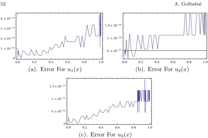
(50) which has the exact solution u1(x) =x2, u2(x) =x and u3(x) = 3x2. Fig-ure.1 show the absolute error when we apply our method for M = 3 and
k= 1.
It is clear form figures that our approximate solution is in good agreement with exact one.
Example 5.2. As a second example, consider the nonlinear system given in [2, 1]
u′1(x) = 1−12u′2(x) + ∫x
0 ((x−t)u2(t) +u1(t)u2(t))dt, u′2(x) = 2x+∫0x((x−t)u1(t)−u22(t) +u21(t))dt, u1(0) = 0, u2(0) = 1,
(51)
which has the exact solutionu1(x) =sinh(x) andu2(x) =cosh(x) forM = 6 andk= 1.
0.0 0.2 0.4 0.6 0.8 1.0 0
1.´10-16 2.´10-16 3.´10-16 4.´10-16
0.0 0.2 0.4 0.6 0.8 1.0
5.´10-17 1.´10-16 1.5´10-16
(a). Error Foru1(x) (b). Error Foru2(x)
0.0 0.2 0.4 0.6 0.8 1.0
0 5.´10-16 1.´10-15 1.5´10-15
(c). Error Foru3(x)
Figure 1: Absolute error for Example 5.1 for M=3 And k=1
Example 5.3. Consider the nonlinear fractional order integro differential equation given in[7]
Dα∗tu(t) = 1 + ∫ x
0
u(t)D∗αtu(t)dt 0≤x <10≤α <1 (52) The exact solution of this problem for α= 1 is √2T an(
√ 2
2 t) we solve this equation form= 20 and differentαnumerical results are shown in Figure 2.
Example 5.4. Finally Consider the nonlinear fractional order integro dif-ferential equations in[7]
Dα∗tu(t) =−1 +
∫ x
0
u2(t)dt0≤x <1 0≤α <1 (53)
subject to the initial conditions y(0) = 0. Table 2 shows the numerical results for α = 0.8,0.9,1 when m = 20. From Table 2 we can see that the approximate solutions obtained by our method are in good agreement with the exact solution for α= 1, and with the approximate solutions for
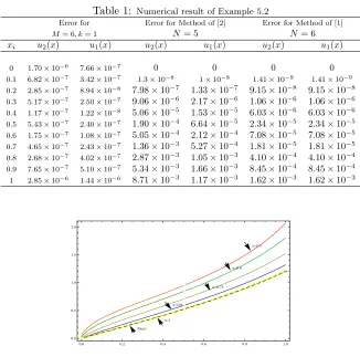
Table 1: Numerical result of Example 5.2
Error for Error for Method of [2] Error for Method of [1]
M= 6, k= 1 N= 5 N= 6
xi u2(x) u1(x) u2(x) u1(x) u2(x) u1(x)
0 1.70×10⁻⁶ 7.66×10⁻⁷ 0 0 0 0
0.1 6.82×10⁻⁷ 3.42×10⁻⁷ 1.3×10⁻⁸ 1×10⁻⁸ 1.41×10⁻⁹ 1.41×10⁻⁹ 0.2 2.85×10⁻⁷ 8.94×10⁻⁸ 7.98×10⁻⁷ 1.33×10⁻⁷ 9.15×10⁻⁸ 9.15×10⁻⁸ 0.3 5.17×10⁻⁷ 2.50×10⁻⁷ 9.06×10⁻⁶ 2.17×10⁻⁶ 1.06×10⁻⁶ 1.06×10⁻⁶
0.4 1.17×10⁻⁷ 1.22×10⁻⁸ 5.06×10⁻⁵ 1.53×10⁻⁵ 6.03×10⁻⁶ 6.03×10⁻⁶ 0.5 5.43×10⁻⁷ 2.40×10⁻⁷ 1.90×10⁻⁴ 6.64×10⁻⁵ 2.34×10⁻⁵ 2.34×10⁻⁵ 0.6 1.75×10⁻⁷ 1.08×10⁻⁷ 5.05×10⁻⁴ 2.12×10⁻⁴ 7.08×10⁻⁵ 7.08×10⁻⁵ 0.7 4.65×10⁻⁷ 2.43×10⁻⁷ 1.36×10⁻³ 5.27×10⁻⁴ 1.81×10⁻⁵ 1.81×10⁻⁵
0.8 2.68×10⁻⁷ 4.02×10⁻⁷ 2.87×10⁻³ 1.05×10⁻³ 4.10×10⁻⁴ 4.10×10⁻⁴ 0.9 7.65×10⁻⁷ 5.10×10⁻⁷ 5.34×10⁻³ 1.66×10⁻³ 8.45×10⁻⁴ 8.45×10⁻⁴ 1 2.85×10⁻⁶ 1.44×10⁻⁶ 8.71×10⁻³ 1.17×10⁻³ 1.62×10⁻³ 1.62×10⁻³
Α=0.5
Exact Α=1
Α=0.9
Α=0.75 Α=0.6
0.0 0.2 0.4 0.6 0.8 1.0 0.0
0.5 1.0 1.5 2.0
Figure 2: Numerical result for Example 5.3 for differentαand m=20
7 Conclusion
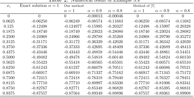
compar-Table 2: Numerical result of Example 5.4
xi Exact solutionα= 1 Our method Method of [7]
α= 1 α= 0.9 α= 0.8 α= 1 α= 0.9 α= 0.8
0 0 0 -0.00013 -0.00046 0 0 0
0.0625 -0.06250 -0.06249 -0.08574 -0.11683 -0.06250 -0.08574 -0.11682 0.125 -0.12498 -0.124977 -0.15995 -0.20327 -0.12498 -0.15997 -0.20328 0.1875 -0.18740 -0.18749 -0.23023 -0.28080 -0.18740 -0.23024 -0.28082 0.2500 -0.24968 -0.24966 -0.29788 -0.35269 -0.24968 -0.29790 -0.35272 0.3125 -0.31171 -0.31172 -0.36339 -0.42026 -0.31171 -0.36342 -0.42039 0.3750 -0.37336 -0.37333 -0.42695 -0.48409 -0.37336 -0.42689 -0.48413 0.4375 -0.43446 -0.43443 -0.48858 -0.54446 -0.43446 -0.48861 -0.54451 0.5000 -0.49482 -0.49478 -0.54818 -0.60140 -0.49482 -0.54824 -0.60150 0.5625 -0.55423 -0.55418 -0.60565 -0.65501 -0.55423 -0.60571 -0.65510 0.6250 -0.61243 -0.61237 -0.66078 -0.70511 -0.61243 -0.66086 -0.70521 0.6875 -0.66917 -0.66910 -0.71337 -0.75162 -0.66917 -0.71345 -0.75172 0.7500 -0.72415 -0.72418 -0.76318 -0.79440 -0.72415 -0.76327 -0.79451 0.8125 -0.77710 -0.77710 -0.80997 -0.83330 -0.77710 -0.81006 -0.83341 0.8750 -0.82767 -0.82771 -0.85348 -0.86820 -0.82767 -0.85395 -0.86831 0.9375 -0.87557 -0.87564 -0.89349 -0.89896 -0.87557 -0.89361 -0.89908
ison with other methods. This procedure can also be used for solving other functional equations such as ordinary and partial differential equations.
References
1. Abbasbandy, S. and Taati, A.Numerical solution of the system of nonlin-ear Volterra integro-differential equations with nonlinnonlin-ear differential part by the operational Tau method and error estimation, journal of compu-tational and Applied Mathematics, 231(2009)106-113.
2. Biazar, J., Ghazvini, H. and Eslami, M. He’s homotopy perturbation method for systems of integro-differential equations, Chaos Solition and Fractals, doi:10.1016/j.chaos.2007.06.001.
3. Caputo, M. Linear modles of dissipation whose Q is almost frequenty independent, Part II, J.Roy. Astr. Soc.,13:529-539.
4. El-shahed, M. Application of He,s homotopy perturbation method to Volterra,sintgro-differential equation, International Journal of Nonlinear sciences and Numerical Simulation 8 (2) (2007) 223-228.
5. Elsayed, S. M., Kaya, D. and Zarea, S.The decomposition method applied to solve high order linear Volterra-Fredholm integro-differential equations, International Journal of Nonlinear sciences and Numerical Simulation 8 (2) (2007) 211-222.
equa-tion, Communication in Nonlinear sciences and Numerical Simulation 16 (2011) 1356–1362.
7. Gazanfari, B., Ghazanfari, A. G. and Veisif, F. Homotopy perturbation Method for the nonlinear fractional integro differentioal equations, Aus-tralian Journal of Basic an Applied Sciencec 4 (12) (2010) 5823-5829.
8. Golbabai, A. and Javidi, M.Application of He’s homotopy perturbation method for n-th order integro differential equations, Applied Mathematics and Computation, 190 (2007) 1409-1416.
9. Golbabai, A. and Javidi, M.A numerical solution for solving system of Fredholm integral equation by using perturbation method, Applied Math-ematics and Computation, 189 (2007) 1921-1928.
10. Guf, J. S. and Jiang, W. S. The Haar wavelet operational m atrix of integration, International Journal of Systems Science, 27 (1996) 623-628.
11. Hu, X. B. and Wu, Y. T.Application of the Hirota bilinear formalism to a new integrable differential-difference equation, Physics Letters A, 246 (1998) 523-529.
12. Kilicman, A. and Al Zhour, Z. A. A.Kronecker operational matrices for fractional calculus and some application, Applied Mathematic and Com-putation 187(2007)250-265.
13. Liu, N. and Ling, E. B.Legendre wavelets method for numerical solutions of partial differential equations, Numerical Methods for partial Differen-tial Equations. 26 (2009) 81-94.
14. Podlubny, I.Fractional differential equations:an introduction to fractional derivatives, fractional differentional equations, to methods of their solu-tion and some their applicasolu-tion. New York: Academic Press; 1999.
15. Razzaghi, M. and Yousefi, S. Legendre wavelets method for constrained optimal control problems, Mathematical method in Applied Sciences. 25 (2002)529-539.
16. Razzaghi, M. and Yousefi, S. Legendre wavelet method for the nonlin-ear Volterra-Fredholm integral equations, Mathematics and Computer in Simulation. 70 (2005) 1-8.
17. Razzaghi, M. and Yousefi, S. Legendre wavelets direct method for vari-ational problems, Mathematics and Computer in Simulation. 53 (2000) 185-192.
19. Rehman, M. and Ali Khan, R.The Legendre wavelet methosd for solving fractional differentional equations, Communication in Nonlinear sciences and Numerical Simulation 16 (2011) 4163-4173.
20. Sun, F. Z., Gao, M., Lei, S. H., Zaho, Y. B., Wang, K., Shi, Y. T. and Wang, N. H.The fractal dimension of the fractal model of dropwise con-densation and its experimental study, International Journal of Nonlinear sciences and Numerical Simulation 8 (2) (2007) 211-222.
21. Taghvafard, H. and Erjaee, G. H.On solving a system of singular Volterra integral equations of convolution type, Communication in Nonlinear sci-ences and Numerical Simulation 16 (2011) 3486–3492.
22. Tarasov, V. E.Fractional integro diffe rentional equations for electromag-netic waves in dielectric media, Theoritical and Mathematical Physics, 153 (3) (2009) 355-359.
23. Wang, H., Fu, H. M. , Zhang, H. F. and Hu, Z. Q. A practical thermo-dynamic method to calculate the best glass-forming composition for bulk metallic glasses, International Journal of Nonlinear sciences and Numer-ical Simulation 8 (2) (2007) 171-178.