Electricity Demand in MENA Countries:
A Panel Cointegration Analysis
Mohammad Sharif Karimi*1 Huseyin Karamelikli2
Received: 2016/02/21 Accepted: 2016/05/01
Abstract
n this study, we applied recently developed panel unit root and cointegration techniques to examine the long-run real income per capita and price elasticities for demand of electricity in selected Middle East and North African (MENA) countries using an annual data series from 1990 to 2011.Our main finding from the panel analysis is that the demand for electricity is highly price elastic and slightly income elastic in the long run for MENA countries. Our findings are consistent with the argument that the demand for electricity in the MENA countries is affected largely by strong economic growth.
Keywords: Demand for Electricity, MENA, Panel Cointegration.
JEL classification: Q41, C31.
1.
Introduction
Energy demand modeling is an essential component for energy planning, formulating strategies, and recommending energy policies. Since the early 1970s, when energy caught the attention of policymakers in the aftermath of the first oil crisis, the research on energy demand analysis has vastly increased from a limited understanding of the nature of energy demand and demand response due to the presence of external shocks in the 1970s.
Electricity consumption in the MENA region has been increasing steadily for the past 22 years, with a registered annual consumption growth rate of around 19.43% from 1990 to 2011. This increased demand in electricity consumption was due to several social, economic, and climatic changes such as the inflation of the gross domestic product, modernization, and the
1. Assistant Professor, Department of Economics, Faculty of Social Sciences, Razi University, Kermanshah, Iran. ([email protected]).
2. Assistant Professor, Economics Science Department, Karabuk University, Turkey ([email protected]).
development of our society (World Bank Database, 2015). The policy focus on climate change mitigation has led to a resurgence of studies regarding household electricity demand, focused on three distinct issues: understanding price responsiveness, appliance choice, and the effect of policy on energy demand, including the issue of “rebound” effects (Krishnamurthy and Kriström, 2015).
In general, electricity is a matter of particular treatment, and it has very specific usage areas with low substitution possibilities, so it should be handled with meticulous care. Policymakers should know the main factors that influence electricity demand in MENA countries since the degree of their effect on consumption has a very important place in the contemplation of energy policy (Gam and Rejeb, 2012). As we know, the construction of new electricity-generating plants requires huge investment and takes a long time to build. Almost all of these plants consume water and oil. Since we seek to reduce the demand of energy and water, while also satisfying population needs at the same time, we need effective electricity management in terms of both production and consumption.
There are a few studies that have estimated income and price elasticities for residential electricity within a panel framework utilizing pooled cross-sectional and time series state-level data within the MENA, and some studies that examine the demand for a range of energy products across the Middle East (for example, Al-faris, 1997). These studies, however, have not first tested whether the panel data are stationary, so the findings are potentially spurious. To test whether there is a long-run relationship between residential electricity demand and its determinants, the panel cointegration test of Pedroni (2004) is used which has the advantage that it allows for heterogeneity across countries.
The outline of the paper is as follows: We lay out the econometric approach and discuss the effects of using average price in Section 2; in Section 3, we provide a few survey details and summary statistics of data used in the regression. Results of estimation are provided and discussed in the context of existing literature in Section 4, while Section 5 concludes with a discussion of our results within a policy context.
2. Economic growth and electricity consumption in MENA
Kuwait, Iran, Iraq, Qatar, United Arab Emirates, and Saudi Arabia benefited directly in the form of higher oil export earnings. The other Middle East states such as Jordan, Yemen, and the Palestinian areas benefited through transmission mechanisms from the oil producer states including labor remittances and aid (World Bank, 2015). Bahrain, which only has a small oil reserve, turned itself into an international banking center, attracting a large amount of the area’s petrodollars (Al-Iriani, 2006). The high rates of economic growth in the 1970s and early 1980s started to fall following the gradual decline in oil revenues from 1983. Real GDP in the MENA region grew at an average of 2.7% per annum between 1985 and 1994. However, in more recent years, these regions have benefited from rising oil prices and OPEC oil production increases. Since income also increased in these countries, the use of energy especially electricity has also increased rapidly. Electricity consumption rose dramatically in the MENA region between 1990 and 2011, more than quadrupling from 169 bkWh to 978 bkWh. The region’s rapidly rising electricity demand (9.7% per year) reflects both the population growth, particularly in the Persian Gulf and North African states, and the higher per capita electricity consumption rates.
Fig. 1. Electric Power Consumption (Kwh)
Sources: WDI(2015)
3. Literature Review
Bentzen and Engsted (1993) had used Danish annual data of real income and real price of electricity from 1948 to 1990 to estimate the impact of real income on the real price of electricity in the short and long run. To explain the directions of relationships between electricity consumption, real income, and employment in Australia, Narayan and Smyth (2005) had used Granger causality tests. Halicioglu (2007) estimated the residential electrical demand in Turkey using annual data covering the period between 1968 and 2005. In his paper, Halicioglu sought to determine relationships for the impact of real income and the urbanization rate on the residential electricity demand and electricity price. In his paper, Erdogdu (2007) remarked that the changes in the price of electricity and income had a limited effect on electricity demand. There were few studies that used monthly or quarterly data to determine the relationship. Tserkezos (1992) estimated the residential electricity consumption in Greece by using both monthly and quarterly data between January 1975 and December 1989. The different findings in the literature can also be explained by examining explicative variables. A few researchers such as Bentzen and Engsted (1993), Galindo (2005), Erdogdu (2007), and
Mabugu et al. (2009) have sought to determine the effect of real income and
relative energy price on the energy demand for consumption. Temperature is a very important factor that influences energy consumption and should be taken into account. Tserkezos (1992), Silk and Joutz (1997) and Amarawickrama and Hunt (2008) added to their model the price of another energy source. They sought to determine the possibility of substitution
0 5E+10 1E+11 1.5E+11 2E+11 2.5E+11 198 5 198 6 198 7 198 8 198 9 199 0 199 1 199 2 199 3 199 4 199 5 199 6 199 7 199 8 199 9 200 0 200 1 200 2 200 3 200 4 200 5 200 6 200 7 200 8 200 9 201 0 201 1
between electricity energy and other energy sources. Many other studies such as Donatos and Mergos (1991) and Narayan and Amyth (2005) were interested in determining the possibility of substitution. In their study, Holtedahl and Joutz (2004) established a model to determine the residential electricity demand in Taiwan using annual data between 1955 and 1995. They sought to quantify the impact of the real price of electricity, the real income, the world price of oil, urbanization, and temperature on the residential electricity consumption both for short and long terms. The variable of urbanization is used to approximate the variable of “Equipment” that is quantified with difficulty. Thanks to this variable that is found easily through statistics, the model is easily estimated. In this context, the “Equipment” variable fits our study. We want to resume the studies of the previous researchers and to analyze the electricity demand for MENA countries as well.
4. Model Specification
The model considered in this paper is based on a typical equation adopted to analyze the demand for electricity. In order to obtain an overall picture of electricity demand, the model uses only variables expected to have significant explanatory power in all countries.
Specifically, the demand for electricity is explained by the consumer's allocation of expenditures among three main categories of goods, namely energy, non-energy domestic goods, and non-energy imported goods, given
the income level and prices, as discussed in Pesaran et al. (1998). The
inclusion of a time trend in the empirical model accounts for the impact of technological trends and shifts towards energy intensive activities associated with factors such as urbanization and industrialization on electricity demand. Electricity consumption and real income are divided by population to yield per-capita series so that demand analysis is carried out in terms of price and income sensitivities for policy purposes. Specifically, population size is one of the factors determining electricity consumption. Also, it allows the comparability of electricity consumption across residential and non-residential sectors and across countries. At a later stage, the per-capita consumption series will be multiplied by the projected population to compute the forecasts of total electricity demand in each sector (see Pesaran et al., 1998).
Then, our model is specified as follows:
𝑙𝑛𝑞𝑖𝑡 = 𝛼𝑖+ β𝑖1𝑙𝑛𝑝𝑖𝑡+ β𝑖2𝑙𝑛𝑦𝑖𝑡+ β𝑖3𝑙𝑛𝐺𝑃𝑖𝑡+ β𝑖4𝑙𝑛𝑝𝑜𝑝𝑖𝑡+ 𝜀𝑖𝑡 (1)
log of residential electricity consumption per capita (Kwh per capita), lnP is the natural log of the real residential electricity price ($US/kWh). The expected sign on the electricity price is negative; lnY is the natural log of real income per capita. Higher real income per capita is expected to increase electricity consumption through greater economic activity and hence increase purchases of electrical equipment. ln GP is the natural log of the real price of natural gas. The nominal prices are deflated by the consumer price index. An increase in the price of gas is expected to generate an increase in the consumption of electricity since gas is a substitute good. lnPOP is the country population which is expected to have a positive effect
on electricity consumption.
𝛼
𝑖 are section effects, i denotescross-sectional units, t denotes time, and the disturbance
𝜀
𝑖𝑡 is assumed to beindependently distributed with an expected value of zero and finite heterogeneous variance σi. It has the property that the β parameters can be interpreted as elasticity, which are of particular interest in demand studies.
5. Methodology
5.1. Panel Unit Root Test
The starting point is to examine whether [q, y, p, gp, pop] contain a panel unit root. While a number of panel unit root tests have been developed, in this study, we have used the panel unit root test proposed by Breitung (2000). The reason for using the Breitung (2000) panel unit root test is that a recent large-scale Monte Carlo simulation study by Hlouskova and Wagner (2006) found that the Breitung (2000) panel unit root test generally has the highest power and smallest size distortions among all the so-called first generation panel unit root tests.
A model developed by Breitung (2000) is a panel unit root test. Since that is achieved by appropriate variable transformations, the panel unit root test does not require bias correction factors. Unit root tests explain the null hypothesis that the process is non-stationary. On the other hand, the alternative hypothesis is that the panel series is stationary. A t-test statistic proposed by Breitung (2000) tests the null hypothesis. The t-test statistic has a standard normal distribution. The Breitung (2000) panel unit root test is based on Eq. (2).
𝑌𝑖𝑡 = 𝜇𝑖𝑡+ ∑ 𝑝+1
𝑖=1
𝛽𝑖𝑘𝑥𝑖,𝑡−𝑘+ 𝜀𝑡 (2)
The test statistic examines the null hypothesis that the process is
𝐻0: ∑ 𝑃+1
𝐾=1
𝛽𝑖𝑘𝑘−1= 0 (3)
𝐻1: ∑ 𝑃+1
𝐾=1
𝛽𝑖𝑘𝑘−1< 1 (4)
In our model, if our variables [q, y, p, gp, pop] contain a panel unit root, the issue arises whether there exists a long-run equilibrium relationship between the variables. We use the Pedroni (2004) test to examine for panel cointegration that allows both for heterogeneity in the intercepts and slopes of the cointegrating equation. In his test, Pedroni (2004) provides seven statistics to test the null hypothesis, which means no cointegration in heterogeneous panels. One part of seven statistics is entitled “within dimension” which takes into account common time factors and allows for heterogeneity across countries. The other part is termed “between dimension” that allows for heterogeneity of parameters across countries. The established seven statistics by Pedroni (2004) that we employ are as follows:
Within dimension (panel tests): a) Panel v-statistic
b) Panel Phillips–Perron type r-statistics. c) Panel Phillips–Perron type t-statistic.
d) Panel augmented Dickey–Fuller (ADF) type t-statistic. Between dimension (group tests):
e) Group Phillips–Perron type r-statistics. f) Group Phillips–Perron type t-statistic. g) Group ADF type t-statistic.
These seven statistics are based on the estimated residuals as used by Pedroni (2004), which we obtain from the Eq. (1) panel cointegration
regression, where 𝜀𝑖𝑡 = 𝛾𝑖𝜀𝑖(𝑡−1)+ 𝜇𝑖𝑡 are the estimated residuals from the
panel regression analysis. In this panel regression, the null hypothesis tested
whether
𝛾
𝑖𝑡 is equal to unity. Pedroni (2004) has tabulated the finite sampledistribution for the seven statistics using Monte Carlo simulations. If the test statistics exceed the critical values that were appointed by Pedroni, the null hypothesis of no cointegration is rejected, implying that a long-run relationship exists between [q, y, p, gp, pop].
6. Data
The 15 countries in the sample are Bahrain, Iran, Iraq, Lebanon, Jordan, Kuwait, Oman, Qatar, Saudi Arabia, Syria, UAE, Tunisia, Egypt, Morocco and Yemen. Annual data from 1990 until 2011 were derived from the International Energy Agency, the World Development Indicators of the World Bank.
Our measure of the demand for electricity, consistent with previous similar studies, is aggregate domestic demand for electricity measured in KW per hour. In order to obtain the real electricity price P, the nominal prices are deflated by Consumer Price Index for all countries obtained from the World Bank, whilst real income is measured in US dollars at 1995 prices based on purchasing power parity; and the electricity price is measured in US dollars per kwh; population is introduced as market size for electricity and consumption of natural gas is introduced as a separate variable where it is treated as a substitute source of energy. This is the most common approach in the literature that models the price of a substitute source of energy. Data were obtained from the World Bank, specifically from WDI 2015. All data were converted into natural logarithmic form prior to conducting the analysis.
7. Empirical Results
A prerequisite for implementing the Pedroni (2004) panel cointegration test is to establish that [q, p, y, x] contains a panel unit root.
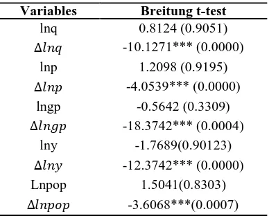
We applied the Augmented Dickey fuller (ADF) test to each individual country. The results are not reported in this paper, but the results of unit root test indicate that the series of each country for all variables contained a unit root. Table 1 reports the Breitung t-test results that were applied to [q, y, p, gp, pop] for the panel of 15 countries. The results show that each of [q, y, p, gp, pop] contains a panel unit root.
Table 1. Panel unit root test Variables Breitung t-test
lnq 0.8124 (0.9051)
∆𝑙𝑛𝑞 -10.1271*** (0.0000)
lnp 1.2098 (0.9195)
∆𝑙𝑛𝑝 -4.0539*** (0.0000)
lngp -0.5642 (0.3309)
∆𝑙𝑛𝑔𝑝 -18.3742*** (0.0004)
lny -1.7689(0.90123)
∆𝑙𝑛𝑦 -12.3742*** (0.0000)
Lnpop 1.5041(0.8303)
∆𝑙𝑛𝑝𝑜𝑝 -3.6068***(0.0007)
The results suggest that residential electricity consumption, real income per capita, the real electricity price, the natural gas price and the population are integrated of order one. We are able to reject the joint unit root null hypothesis for all the five variables at the 1% level of significance. We proceed to examine whether there is a long-run relationship between residential electricity consumption and its determinants employing the Pedroni (2004) panel cointegration test and using the three group-based test statistics. The results are reported in Table 2. Test statistics suggest that there is panel cointegration among the variables for the MENA countries. We find that test statistics reveal evidence of panel cointegration at either the 5% or 1% level of significance.
Table 2. Pedroni’s (2004) panel cointegration test
Panel v-statistic -4.9291** (0.0002)
Panel Phillips–Perron r-statistic 3.1065** (0.0123)
Panel Phillips–Perron t-statistic 2.0629** (0.0884)
Panel ADF t-statistic 2.1462** (0.0480)
Group Phillips-Perron r-statistic 3.9602*** (0.0073)
Group Phillips–Perron t-statistic 8.003*** (0.0000)
Group ADF t-statistic 2.0054** (0.0190)
Notes: Probability values are in parenthesis; ** and *** denote statistical significance at the 5 percent and 1 percent levels, respectively.
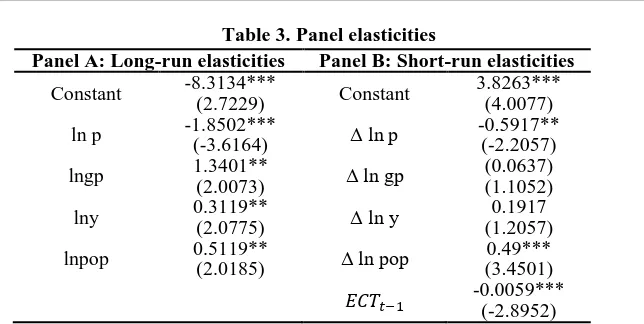
Table 3. Panel elasticities
Panel A: Long-run elasticities Panel B: Short-run elasticities
Constant -8.3134***
(2.7229) Constant
3.8263*** (4.0077)
ln p -1.8502***
(-3.6164) Δ ln p
-0.5917** (-2.2057)
lngp 1.3401**
(2.0073) Δ ln gp
(0.0637) (1.1052)
lny 0.3119**
(2.0775) Δ ln y
0.1917 (1.2057)
lnpop 0.5119**
(2.0185) Δ ln pop
0.49*** (3.4501)
𝐸𝐶𝑇𝑡−1 -0.0059*** (-2.8952)
Notes: t-statistics are in parenthesis;*, **, and *** denote statistical significance at the 10, 5, and 1 percent levels, respectively.
The panel long-run elasticity for the electricity price variable is -1.85 implying that a 1% increase in the electricity price reduces residential electricity consumption by around 1.8% in the long-run. Also, the long-run panel cross-price elasticity with natural gas is 1.34, meaning that a 1% increase in natural gas prices increases electricity consumption by between 1.3% in the long-run. In addition, long –run elasticities for population and GDP per capita are 0.51 and .0311. On the other hand, the short-run price elasticity is much lower than the long-run price elasticity, and in this period, a 1% increase in electricity prices reduces residential demand for electricity by 0.59%.
6. Conclusion
References
Al-Faris, A. F. (1997). Demand for Oil Products in the GCC Countries. Energy Policy, 25, 55–61.
Al-Iriani, M. (2006). Energy–GDP Relationship Revisited: an Example from
GCC Countries Using Panel Causality. Energy Policy, 34, 3342–3350.
Amarawickrama, A. H., & Hunt, C. L. (2008). Electricity Demand for
Sri-Lanka: a Time Series Analysis. Energy, 33, 1179–1185.
Bentzen, J., & Engsted, T. (1993). Short and Long-Run Elasticities in
Energy Demand: a Co-Integration Approach. Energy Economics, 15, 9–16.
Breitung, J. (2000). The local Power of Some Unit Root Tests for Panel Data. In: Baltagi, B.H. (Ed.), Nonstationary Panels, Panel Co-integration and
Dynamic Panels. Elsevier, Amsterdam, 161–177.
Chandra, Kiran, Krishnamurthya, B., & Bengt, Kriström (2015). A Cross-Country Analysis of Residential Electricity Demand in 11 OECD-Countries. Resource and Energy Economics, 39, 68–88.
Erdogdu, E. (2007). Electricity Demand Analysis Using Co-Integration and
ARIMA Modelling: a Case Study of Turkey. Energy Policy, 35, 1129–1146.
Gam, I., & Rejeb, J. B. (2012). Electricity Demand in Tunisia. Energy
Policy, 45, 714-720.
Galindo, L. M. (2005). Short-and Long-Run Demand for Energy in Mexico:
a Co-Integration Approach. Energy Policy, 33, 1179–1185.
Halicioglu, F. (2007). Residential Electricity Demand Dynamics in Turkey. Energy Economics, 29, 199–210.
Imen Gama, N., & Rejeb, Jaleleddine Ben (2012). Electricity demand in
Tunisia. EnergyPolicy, 45, 714–720.
Holtedahl, P., & Joutz, F.L. (2004). Residential Electricity Demand in
Taiwan. Energy Economics, 26, 201–224.
Hlouskova, J., & Wagner, M. (2006). The Performance of Panel Unit and
Stationary Tests: Results from a Large Scale Simulation Study. Econometric
Reviews, 25, 85–116.
Co-Integrated Regression in Panel Data. In: Baltagi, B. H. (Ed.), Advances in Econometrics, Nonstationary Panels, Panel Co-integration and Dynamic panels, JAI Press, Amsterdam, 15, 179–222.
Mabugu, R., Amusa, H., & Amusa, K. (2009). Aggregate Demand for Electricity in South Africa: an Analysis Using the Bounds Testing Approach
to Co-Integration. Energy Policy, 37, 4167–4175.
Narayan, P. K., & Smyth, R. (2005). Electricity Consumption, Employment and Real Income in Australia Evidence from Multivariate Granger Causality
Tests. Energy Policy, 33, 1109–1116.
Pedroni, P. (2004). Panel Co-Integration: Asymptotic and Finite Sample Properties of Pooled Time Series Tests with an Application to PPP
Hypothesis: New Results. Econometric Theory, 20, 597–627.
Pesaran, M. H., Smith, R., & Akiyama, T. (1998). Energy Demand in Asian
Economies. Oxford, Oxford University Press.
Silk, I. J., & Joutz, L. F. (1997). Short and Long-Run Elasticities in US
Residential Electricity Demand: a Co-Integration Approach. Energy
Economics, 19, 493–513.
Tserkezos, E. D. (1992). Forecasting Residential Electricity Consumption in
Greece Using Monthly and Quarterly Data. Energy Economics, 14, 226–232.