Land Cover Classification Using IRS-1D Data and a Decision Tree Classifier

DESERT 17 (2013) 137-146

Land Cover Classification Using IRS-1D Data and a Decision Tree

Classifier

H.R. Keshtkar

, H. Azarnivand

, H. Arzani

, S.K. Alavipanah

, F. Mellati

a

MSc. Graduate, University of Tehran, Karaj, Iran b

Professor, Faculty of Natural Resources, University of Tehran, Karaj, Iran c

Professor, Faculty of Geography, University of Tehran, Tehran, Iran

d _{Instructor, Faculty of Environment and Natural Resources, Ferdowsi University, Mashhad, Iran}

Received: 16 June 2008; Received in revised form: 10 December 2008; Accepted: 22 January 2009

Abstract

Land cover is one of basic data layers in geographic information system for physical planning and environmental monitoring. Digital image classification is generally performed to produce land cover maps from remote sensing data, particularly for large areas. In the present study the multispectral image from IRS LISS-III image along with ancillary data such as vegetation indices, principal component analysis and digital elevation layers, have been used to perform image classification using maximum likelihood classifier and decision tree method. The selected study area that is located in north-east Iran represents a wide range of physiographical and environmental phenomena. In this study, based on Land Cover Classification System (LCCS), seven land cover classes were defined. Comparison of the results using statistical techniques showed that while supervised classification (i.e. MLC) produces an overall accuracy of about 72%; the decision tree method, which improves the classification accuracy, can increase the results by about 7 percent to 79%. The results illustrated that ancillary data, especially vegetation indices and DEM, are able to improve significantly classification accuracy in arid and semi arid regions, and also the mountainous or hilly areas.

Keywords: Land cover classification system (LCCS); IRS-1D satellite; Maximum likelihood; Ancillary data

1. Introduction

Land cover is a critical variable in epidemiology and can be characterized remotely. Land cover and land use are principal factors, in both space and time, controlling the cycling and exchange of carbon, energy and water within, and between the different earth systems (Brown de Colstoun and Walthall, 2006). Thus, land cover classification are essential for a variety of diagnostic and predictive models that simulate the functioning of the earth systems and are useful for investigating regional and global change (Brown

 Corresponding author. Tel.: +98 26 32223044, Fax: +98 26 32223044.

E-mail address: [email protected]

sensed data (Richards, 1993). This methodology assumes that the probability distributions for the input classes possess a multivariate normal form. Increasingly, nonparametric classification algorithms such as decision trees (DT) are being used, which make no assumptions regarding the distribution of the data being classified (Carpenter et al, 1999; Foody, 1997; Friedl et al, 1999). The nonparametric properly means that non-normal, non-homogenous and noisy data sets can be handled, as well as non-linear relations between features and classes, missing values and both numeric and categorical inputs (Quinlan, 1993). DT classifiers have not been as widely used within the remote sensing community. The advantages that DT offer include an ability to handle data measured on different scales, lack of any assumptions concerning the distributions frequency of the data in each of the classes, flexibility, and ability to handle non-linear relationships between features and classes (Friedl & Brodley, 1997).

The study has two objectives; first, to investigate the ability of two classification methods (i.e., MLC and DT) to separation various land cover classes; secondly, to evaluate performance of ancillary data for improve image classification.

2. Background

2.1. IRS-1D Satellite

The IRS-1D satellite is the fourth in a series of commercial Indian satellites. It was launched in 1997. For the IRS satellite the imaging time is around 10:00 a.m. every 24 days. Onboard the IRS-1D satellite is several sensors one of which the LISS-III. This sensor covers an area of 141×141 km in its scene. Each pixel is 23.5×23.5 m in the raw image data but here resampled to a 24×24 m. LISS-III is a four-band multispectral sensor with narrow bands: 0.52-0.59 µm (green), 0.62-0.68 µm (red), 0.77-0.86 µm (near infrared), 1.55-1.70 µm (middle infrared). A subset of a 2003 image from LISS-III sensor for the growing season (5 May) which includes the study area has been used.

2.2. Maximum likelihood classifier

It is believed that the MLC procedure is based on the assumption that the members of each class follow a Gaussian frequency distribution in

feature space. MLC is a pixel-based method, and can be defined as follows: a pixel with an associated observed feature vector x is assigned to class c_j of N classes if

g_j(x) > g_k(x) for all j≠k, with j,k = 1,…, N. For the multivariate Gaussian distribution, the discriminating function g_k(x) is given by:

gk(x) = ln(p(x | cj)) = lnΣk + (x - µk)TΣ-1 (x - µk) Where µ_k and Σ_k are the sample mean vector and sample covariance matrix for class k.

Implementation of the MLC algorithm involves the estimation of class mean vectors (µ_k) and covariance matrices (Σ_k) from training data selected from known examples of each particular class. The function g_i(x) is used to evaluate the membership probability of an unknown pixel for class j. The pixel is assigned to the class for which it has the highest membership probability value.

2.3. Decision tree classifier

In the usual approach to classification, a common set of features is used jointly in a single decision step. An alternative approach is to use a multistage or sequential hierarchical decision scheme. The basic idea involved in any multistage approach is to break up a complex decision into a union of several simpler decisions, hoping the final solution obtained in this way, would resemble the intended desired solution. Hierarchical classifiers are a special type of multistage classifier that allows rejection of class labels at intermediate stages.

A tree is composed of a root node (containing all the data), a set of internal nodes (splits), and a set of terminal nodes (leaves). Each node in a decision tree has only one parent node and two or more descendent node (Fig 1). A data set is

classified by moving down the tree and sequentially subdividing it according to the decision framework defined by the tree until leaf is reached.

Fig. 1. A classification tree with four dimensional feature space and three classes.

The xi are feature values; a, b, c, d, and e are the thresholds and A, B, and C are class labels (Pal and Mather, 2003).

3. Material and methods

3.1. Study area

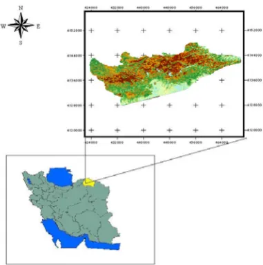
The study was carried out in Ghorkhood region that is a protected area located in north-east of Iran (950-3000 m a.s.l., 43000 ha, see Fig. 2). This area comprises of different landscape unit, including valley bottoms and ravines, plateaus with different degree of dissection and rocky hilly uplands. The climate is cold semi-arid, with an annual average temperature of 13°C, and a mean

annual precipitation of 360 mm (Keshtkar, 2008). In the study area 31 families, 118 genera and 196 species were identified. The largest family is Poaceae with 17 genera and 32 species. The life form of plant species are including 11.2% phanerophytes, 16.8% chamaephytes, 43.9% hemicryptophytes, 8.2% geophytes and 19.9% therophytes (Keshtkar et al, in press), and the most important plant species in the area included: Artemisia sieberi, Salsola aucheri, Juniperus polycarpos, Bromus danthonia, Poa bolbosa, Festuca ovina and Acantholimon festucaceum.

Fig 2. Location and land cover map (created using MLC) of the study area in north east of Iran X1 ≤a

X2 ≤b X3≤d

X2 ≤c X4 ≤e

A B

A C

3.2. Field sampling

From May 5 to May 12, 2003 we took samples of terrain characteristic in 280 selected points. These points were defined as areas of 24×24 m (equivalent to the IRS-1D pixel), around the point located with the GPS (Global Positioning System). Since the beginning of the grazing season in the region is at June of each year, the image of May 5th was selected when the plant species were in active growth stage, which was the best time if we wanted to carry out the field sampling when the vegetation was still fresh. In lands containing natural vegetation cover we recorded land cover type, canopy cover, topographic position, slope, aspect and altitude. But in non-natural areas just land cover type and topographical data were recorded.

A classification scheme defines the land cover classes to be considered for remote sensing image classification. Thus, we used Land Cover Classification System (LCCS) that developed by FAO (FAO, 1997) to detection different land cover types. The study area composed of both man-made (Village) and natural regions (forest and non-forested areas). Forest area is included needle leaved evergreen, and Non-forested areas are composed of farm land, shrubland, meadow and barren land. Although some of these areas

were covered with clouds and cloud shadows on the main image.

3.3. Generation of ancillary data

Principal components analysis (PCA), Digital Elevation Model (DEM) and Vegetation Indices (VI) data layers were used as additional bands (referred as ancillary data) to perform and improve DT classification.

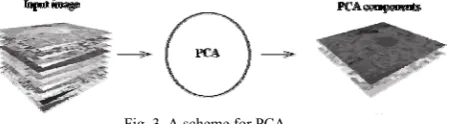
a) Principal Component Analysis

PCA is often used as a method for reducing the number of images (Fig 3). It allows redundant data to be compacted into fewer bands namely the dimensionality of the data is reduced (Jensen, 1996; Faust, 1989). The first components of PCA was used for distinguish and mask shades in the image. Following Jensen (1996) percentage of total variance for each component was calculated as:



 _N

pc pc pc

1 100 var

%

 

Where λPC is eigenvalue that is the variance of the Principal Component PC; N is the number of Principal Components.

Fig. 3. A scheme for PCA

b) Production of DEM and slope maps

DEM was originally a term reserved for elevation data provided by the USGS, but it is now used to describe any digital elevation data. We produced DEM layer by digital topographic maps at a scale of 1:25,000 with 10 m contour interval. Triangulated Irregular Network model was used to produce a raster DEM at 23m spatial resolution to match with that of LISS-III image. Secondary location information derived from DEM includes slope layer. Using DEM map is the best way to prepare this map. Since the region’s gradient is one of determining factors in distribution of plant types, preparing such a map is of significant importance.

c) Calculation of VI

Table 1. Various vegetation indices used in this study and their formulas

Formula Definition

Nomenclature

NIR-RED Deference Vegetation Index

DVI

ŋ (1-0.25)-(R-0.125) / 1-R

ŋ=[2(NIR2-R2)+1.5NIR+0.5R]/(NIR+R+0.5) Global Environmental Monitoring Index

GEMI

(NIR-GREEN)/(NIR+GREEN) Green Normalized Difference Vegetation Index

GNDVI

NIR/(NIR+RED) Infrared Percentage Vegetation Index

IPVI

NDVI/(3.26-2.9+NDVI) Leaf Area Index

LAI

(NIR-MIR)/(NIR+MIR) Leaf Water Content Index

LWCI

(MIR-RED)/(MIR+RED) MIRV

MIRV

(NIR-RED)*(1+L)/(NIR+RED+L) L=1-(2*a*NDVI*WDVI) Modified Soil Adjusted Vegetation Index

MSAVI

MIR/NIR Moisture Stress Index

MSI

(NIR-RED)/(NIR+RED) Normalized Difference Vegetation Index

NDVI

(NIR-RED)/RED NRR

NRR

(RVI-1)/(RVI+1) Normalized Ratio Vegetation Index

NRVI

(RED-GREEN)/(RED+GREEN) PD322

PD322

NIR/(RED+MIR) RA

RA

NIR/RED Ratio Vegetation Index 1

RVI 1

Sqrt (NIR/RED) Ratio Vegetation Index 2

RVI 2

(NDVI+1)*100 Transformed Normalized Difference Vegetation Index

TNDVI

a (NIR-a * RED+b)/RED+a * NIR-a*b Transformed Soil Adjusted Vegetation Index

TSAVI

(NIR-RED)/(NIR+RED)+0.5 Transformed Vegetation Index

TVI

RED*NIR/GREEN Vegetation Index 1

VI 1

RED*NIR Vegetation Index 2

VI 2

3.4. Preparing image

Geometric distortions manifest themselves as errors in the position of a pixel relative to other pixels in the scene. It is very necessary in mountainous areas where distortion can be high due to the steep relief. A series of pre-processing procedures were performed on the images before their categorization. In the first stage, a two dimensional geometric correction was performed on the bands using the Polynomial method (nearest neighbor algorithm for resampling), achieving a positional error of 0.56 of a pixel (13.2 m), with an output pixel size of 24×24 m. The orthorectification was then performed on the image using the DEM and the Rational Function method because the region was mountainous and the research area was located at the periphery of the window which intensifies the displacement phenomenon due to the terrain’s ups and downs. Since the SWIR band has 70 m spatial resolution, while the other bands have 24 m spatial resolution, we resized the SWIR band to create 24 m data to the same size as the other data. Atmospheric corrections were found unnecessary since we used single image for all further analyses and classifications (Song et al, 2001).

3.5. Image classification

The aim of the classification is to categorize all of the pixels in the IRS-1D satellite image

(LISS-III sensor) into land cover classes. The basic assumption is that pixels with similar spectral properties belong to a certain type of land cover, and to do so the MLC and DT procedures are used in this study. For more information a brief summary of the properties of each of these methods is given in background section. In addition to raw bands, we used the PCA, DEM and VI as ancillary data layers for improves to classify image. In order to perform a reliable image classification the class separability need to be enhanced. For this reason, we used a well established measure called the Bhattacharyya distance (Richards & Jia 1999) to quantify the separation between training data classes. The training samples were then reviewed based on the obtained results and their size, distribution and numbers were modified. This operation was repeated several times in order to select the best samples.

3.6. Accuracy estimation

whereas the other two measures indicate the accuracy of individual classes. User’s accuracy is regarded as the probability that a pixel classified on the map actually represents that class on the ground or reference data, whereas producer’s accuracy represents the probability that a pixel on reference data has been correctly classified. To determine the accuracy of classification, a number of randomly selected points measured in the field survey to the accuracy assessment of the classification. The field sample locations were overlaid on classified maps to assess corresponding classes. Statistically valid sampling strategy was adopted to assess overall accuracy (Stehman, 1996). Finally, the contingency table was tested using Kappa coefficient (Lillesand & Kiefer, 1999). Kappa coefficient computed as follows:







xii= The No. of observations in row i and column i (on the major diagonal)

xi+= Total observation in row i (shown as marginal total to the right of the matrix)

x+i= Total observation in column i.

Geomatica 9 and ArcGIS 9.1 software were used to carry out the required processing and analyses on satellite images and digital maps. All statistical analyses have been performed using the statistical software Minitab 13, and the LCCS 2.4 software was used for the execution of FAO model.

4. Results

The results depicts that the most slopes in the study area are covered with trees. In the mountain valleys, a patchwork of meadow and shrubland was observed at intermediate altitudes while at higher altitudes meadow prevailed. Although there are differences in forest composition between north ward and south ward slopes, we suggest that the observed differences in forest composition are largely anthropogenic in origin. These differences are most likely a legacy of socialist forest management practices and policies, because almost all forests were harvested at least once in the 20th century. Finally, according to LCCS we divided the research area into seven classes which are illustrated in Table 2.

Table 2. Characteristics of land cover classes

Description LCCS Code

Land cover class

Mixed woodland 22689-L31M2N2N5O5O11P3Q7

Woodland

Short herbaceous vegetation with dwarf shrubs 21273-12366-M2N2N4O5O11Q6

Meadow

Very stony bare soil 6005-7-L11O5O11P10Q6U2

Bare land

Shifting cultivation of small sized field(s) of herbaceous crop(s) 11248-13227-11O5O11P10Q6W4

Farm land

Low density rural area(s) A4-A13A16-L11O5O11P10

Rural area

Broadleaved deciduous dwarf shrubland with high shrub emergents 20174-12050-M2N2N4O5O11Q6

Open Shrubland

Broadleaved deciduous sparse dwarf shrubs and sparse short herbaceous

20241-6023-L11M2N2N5O5O11P10Q6 Sparse Shrubland

The existing natural complexities in the region and therefore, the blending of pixel have led to the spectral interference between some of the categories. Results that are presented in table 3 indicate the amount of such interferences to some extent (Bhattacharya distance criterion). The lowest separability is related to separation between rural area and bare land. Also, the results depict the separation between sparse shrubland with rural area, barren lands and open shrubland is not easy.

Results also show that the first PCA component has the highest volume of information by having 95.35% of the total information of the bands while other components have 2.58, 1.82 and 0.25% of the share, respectively. Reviewing the

specific coefficient of the first component (PC1) shows that the band 4 has the highest amount of information with a specific coefficient of 0.649 while the band 3 has the lowest share with a specific coefficient of 0.377 (Table 4). Comparing the specific coefficients of the forth component (PC4) for bands 1 and 2 indicate that these two bands are highly correlated.

show that the TSAVI index has the highest correlation (r=0.569, significant level=0.01) with vegetation canopy percentage at sampling spots. Also, a number of other indices namely GEMI,

GNDVI, LWCI, MIRV, MSAVI, NDVI, RVI1 and VI1 have a significant relationship (at significant level=0.05) with vegetation cover.

Table 3. Degree of separation between classes

ME RA FL WL SH CL BL OS

RA 1.7

FL 1.8 1.7

WL 1.4 1.5 1.9

SH 2 2 2 2 CL 2 1.8 2 2 2 BL 1.9 0.6 1.8 1.7 2 2 OS 1.3 1.2 1.7 1.2 2 2 1.2 SS 1.6 0.8 1.7 1.3 2 1.9 1.1 1

Range of variable in this method is between 0-2 that 0 means non-separation, 0-1 means low separation, 1-2 means high separation and 2 means complete separation among classes (ME= Meadow, RA= Rural Area, FL= Farm Land, WL= Wood Land, SH= Shade, CL= Cloud, BL= Bare Land, OS= Open Shrublans and SS= Sparse Shrubland).

Table 4. The statistical results of PCA of LISS-III image

PC1 PC2 PC3 PC4

Green Band 0.474 0.404 -0.094 0.777 Red Band 0.461 0.642 0.120 -0.601 NIR Band 0.377 -0.284 -0.861 -0.187 MIR Band 0.649 -0.586 0.484 -0.032

% Variance 95.35 2.58 1.82 0.25

Cumulative Variance 95.35 97.93 99.75 100

In current study all spectral bands were imported to software for supervised classification by MLC, but different combination data composed of spectral bands along with ancillary data used to separate various classes in DT approach. Finally, the land cover types were separated using the following band combinations: Woodland (Red and NIR bands with DEM and slope map), Bare land (TSAVI index, Red, NIR and MIR bands), Farm land (Red, NIR and MIR bands along with NDVI index and DEM), Meadow (GEMI index along with Red and NIR bands), Open shrubland (TSAVI index, Red and NIR bands), Sparse shrubland (Red and NIR bands with TSAVI index), Cloud (all of bands and DEM) and Shade (the first component of PCA). The overall accuracy and Kappa coefficient of land cover maps obtained from two models used in current study is shown in Table 5. The classification based on MLC produced an accuracy of 70.2%, while the highest accuracy of 79.3% was obtained by the DT approach. To assess the accuracy of individual land cover classes, producer’s and user’s accuracies were also determined for the classified images (Table 6). A glance at producer’s and user’s accuracy values show that the accuracy of most of the classes has increased in DT classification process. This illustrates that the misclassifications between

the classes have been reduced. Classified images often manifest a noisy (salt-and-pepper) appearance. To remove these stray pixels so as to produce smooth land cover classification, a 3×3 majority filter was applied over the two classified images. The resulting product was considered as the final land cover map to be used as input for subsequent GIS based study.

5. Discussion and Conclusion

characteristics of some classes in areas with low vegetation coverage.

The existing natural complexities in the region and therefore, the blending of pixel have led to the

spectral interference between some of the categories. Some of the cases below can also be named as factors creating such interferences:

Table 5. Comparison of classifications obtained from DT and MLC Overall Accuracy (%) Kappa Coefficient

DT 79.3 0.76

MLC 70.2 0.62

Table 6. Producer’s and User’s accuracy (%) of individual classes derived from classified images using DT and MLC methods

MLC DT Land cover class

producer’s accuracy User’s accuracy producer’s accuracy User’s accuracy

Woodland 65 71 74 69

Meadow 58 63 79 81

Bare land 96 71 52 83

Farm land 100 42 92 76

Rural area 0 0 0 0

Open Shrubland 59 50 58 79

Sparse Shrubland 61 84 64 80

Cloud 39 64 100 100

Shadow 100 100 100 100

The existence of understory in woodlands and relatively high distances between trees resulted in most of spectral reflectance of these regions to be allocated to the under-canopy. Therefore, we observed the spectral interference between such lands, woodland, shrublands and meadows. Curran et al (1992), Abuelghasem et al (1999), Mickelson et al (1998) and Nemani et al (1993) had same reports.

Another problem is the spectral interference between open shrubland and sparse shrubland classes. This interference is due to high soil reflectance in these two types, in addition to the existence of similar plants (having similar vegetative types). This causes the soil reflectance to dominate the vegetation reflectance. Uses of soil line indices, especially TSAVI, reduce this problem to some extent. Rondeaux et al (1995) described TSAVI as the best index to estimate the percentage of vegetation canopy. The results of current study confirm this TSAVI is a determining variable in separating three different types (i.e. woodland, open shrubland and sparse shrubland) in DT method. According to Smith et al (1990) if plant cover is lower than 40% than soil effects may prevail over plant effects. Results of a study by Baret & Guyot (1991) also showed that the use of soil line indices in arid and semi-arid region with sparse vegetation, led to good results. The other problem is related to rural regions. The results showed that the separation of rural areas is not easily possible because most of the residential homes in this region are made of thatch

and stone which show exactly similar spectral behavior as that of bare lands. The very small area of this type compared to other types is one of the limiting factors affecting the separation procedure and plays an important role in decreasing the validity of categorization. Since none of the methods used in this study were not able to separate the rural lands, this category was omitted from the final maps (Fig 4).

was improved by 9.1 percent, Kappa coefficient increased by 0.14. In particular, the classes namely open shrubland, sparse shrubland, woodland, farmland and meadow showed a substantial increase in accuracy. At least one explicit reason may be stated for this increase in accuracy. The class woodland was considerably misclassified with the classes’ open and sparse shrublands when only spectral data were used in MLC method. Since, at high elevations, the

presence of these classes is scarce, addition of topographic layers (DEM and slope) reduced this misclassification in DT method. The present study thus highlights the effectiveness of integrating ancillary data with the spectral data to enhance the quality of land cover classifications in mountainous regions. Also, DT is a potentially useful approach to produce meaningful classifications from remote sensing data. Pal and Mather (2003) obtained same result in their study.

Fig. 4. The land cover classification with the highest accuracy (i.e., 79%), produced by DT method

Acknowledgment

Authors would like to thank the Geography Organization of Iran’s Armed Forces for providing the satellite images and the North Khorasan Province General Directorate of Environment for their cooperation in sampling programs. They would also like to thank all the environmental guards of environmental protection outpost of the protected region of Ghorkhood for providing security and escort during the collection of field samples.

References

Abuelghasim, A.A., Ross, W.D., Gopal, S & Woodcock, C.E. 1999. Change detectioning adaptive fuzzy neural networks environmental damage assessment after the Gulf War. Remote Sensing of Environment, 70: 208- 223.

Baret, F. & G. Guyot, 1991. Potentials and limits of vegetation indices for LAI and APAR assessment. Remote Sensing of environment, 35:161-173.

Brown de colstoun, E.C., & C.L., Walthall. 2006. Improving global scale land cover classifications with multy-directional POLDER data and a decision tree classifier. Remote Sensing of Environment, 100: 474- 485.

Carpenter, G. A., Gopal, S., Macomber, S., Martens, S., Woodcock, C. E., & Franklin, J. 1999. A neural network method for efficient vegetation mapping. Remote Sensing of Environment, 70: 326– 338. Curran, P.J., Dungan, J.L & Gholz, H.L. 1992. Seasonal LAI in slash pine estimated with Landsat TM, Remote Sensing of Environment, 39: 3-13.

DeFries, R. S., Hansen, M., Townshend, J. R. G., & Sohlberg, R. 1998. Global land cover classifications at 8 km spatial resolution: The use oftraining data derived from Landsat imagery in decision tree classifiers. International Journal of Remote Sensing, 19: 3141– 3168.

FAO. 1997. Africover Land Cover Classification, FAO, Rome. Fosberg, F.R., 1961. A classification of vegetation for general purposes. Trop. Ecol. 2, 1–28. Faust, N. L. 1989. Image Enhancement. Volume 20, Supplement 5 of Encyclopedia of Computer Science and Technology. Ed. A. Kent and J. G. Williams. New York: Marcel Dekker, Inc.

Foody, G. M. 1997. Fully fuzzy supervised classification of land cover from remotely sensed imagery with an artificial neural network. Neural Computing and Applications, 5 (4): 238– 247.

Hansen, M. C., DeFries, R. S., Townshend, J. R. G., & Sohlberg, R. 2000. Global land cover classification at 1 km spatial resolution using a classification tree approach. International Journal of Remote Sensing, 21: 1331–1364.

Jensen, J. R. 1996. Introductory digital image processing, 2nd edition. Upper Saddle River, New Jersey: Prentice- Hall.

Keshtkar, H.R. 2008. Investigation of the capability of IRS satellite data for land cover mapping. M.Sc. thesis. University of Tehran.

Keshtkar, H.R., Yeganeh, H & Jabarzare, A. In press. Florestic studies and life forms of Ghorkhood pretected area. Iranian Journal of Biology.

Lillesand, T.M., & Kiefer, R. W. 1999. Remote sensing and image interpretation. New York: John Wiley and Sons.

Loveland, T.R., Zhu, Z., Ohlen, D.O., Brown, J.F., Reed, B.C & Yang, L. 1999. An analysis of the IGBP global land-cover characterization process. Journal of the American society for photogrammetric and remote sensing, 65: 1021–1032.

Mickelson, J.G., Civco, D.L & Silander, J.A. 1998. Delineating forestcanopy species in the northeastern United States using multi-temporal TM imagery, Photogrammetric Engineering and Remote Sensing, 64:891-904.

Nemani. R., Pierc. L & Running, S. 1993. Forest ecosystem processes at the watershed scale: Sensitivity

to remotely-sensed Leaf Area Index estimates. International journal of Remote sensing, 14:2519-2534. Pal, M. & Mather, P. M. 2003. An assessment of the effectiveness of decision tree methods for land cover classification. Remote Sensing of Environment, 86: 554-565.

Quinlan, J. R. 1993. C4.5: Programs for machine learning. Morgan Kaufmann, California.

Richards, J. A. 1993. Remote sensing digital image analysis: an intro-duction. New York: Springer-Verlag. Richards, J.A. & Jia, X. 1999: Remote Sensing Digital Image Analysis, Springer-Verlag, Berlin.

Rondeaux, G., M. Steven & F. Baret, 1995. Optimization of soil-adjusted vegetation indices. Remote Sensing of environment, 55:88-107.

Smith, M. O., Ustin, S. L., Adams, J. B. and Gillespie A. R. 1990. Vegetation in desert I. A Regional Measure of Abundance from multi spectral Images, Remote Sensing of Environment. 31:1-26.

Song, C., Woodcock, C. E., Seto, K. C. Lenney, M. P., & Macomber, S. A. (2001). Classification and change detection using landsat TM data. When and how to correct atmospheric effects? Remote sensing of Environment, 75: 230-244.