7. A Modification of Quasi-Newton (DFP) Method for Solving Unconstrained Optimization Problems

(1)

A Modification of Quasi-Newton (DFP) Method for Solving

Unconstrained Optimization Problems

Salah Gazi Shareef

1

, Ahmed Anwer Mustafa

2

1

Deperatment of Mathematics, Faculty of Science, University of Zakho

2_{Deperatment of Mathematics, Faculty of Science, University of Zakho}

Kurdistan Region-Iraq

1. INTRODUCTION

Quasi-Newton methods are recognized today as one of the most efficient ways to solve nonlinear unconstrained or bound constrained optimization problems. These methods are mostly used when the second derivative matrix of the objective function is either unavailable or too costly to compute. They are very similar to Newton's method, but avoid the need of computing Hessian matrices by recurring, from iteration to iteration, a symmetric matrix which can be considered as an approximation of the Hessian. They allow, therefore, the curvature of the problem to be exploited in the numerical algorithm, despite the fact that only first derivatives (gradients) and function values are required. We refer the reader to [4, 5, 10, 11] for further motivation and analysis concerning these now classical algorithms.

In this study we consider the unconstrained minimization problem

(1.1)

where is continuously differentiable. The DFP method for solving (1.1) generates a sequence of iterates { } by

(1.2) where is the current iterative and is a step size., we denote by by , by

and is a search direction, generally descent and generated from either is an approximation to the Hessian of ) or is used to generate the search direction.

.

(1.3)

There are mainly different in the choice of the parameter . Some well-known formulas for given below:

(1.4)

(1.5)

(1.6)

(1.7)

Abstract—

The Quasi-Newton method is a very useful technique for solving minimization problems and has wide applications in many fields. In this paper we develop a new class of DFP method for unconstrained optimization. The given method satisfies the Quasi-Newton condition and positive definite theorem under strong Wolfe line search. Numerical results based on the number of iterations (NOI) and number of function (NOF), have shown that the new method (New5) performs better than standard method of ( ) method.

Keywords

—

Unconstrained optimizations, DFP method, Quasi-Newton condition, positive definite

(2)

(1.8)

(1.9)

(1.10)

(1.11)

(1.12)

(1.13)

where and g are the gradients of at the point and respectively.The above corresponding methods, HS is known as Hestenes and Steifel [6], FR is Fletcher and Reeves [8], PR is Polakand Ribiere [3], CD is Conjugate Descent [9],BA2 is AL - Bayati, A.Y. and AL-Assady[2],

LS is Liu and Storey [14], DY is Dai and Yuan [13], HZ is Hager and Zhang [12], M. Rivaie, A. Abashar, M. Mamat and I. Mohd[7] and lastly AMRI denotes Abdelrhaman Abashar, Mustafa Mamat, Mohd Rivaie and Ismail Mohd[1].

The matrix is required to satisfy the Quasi-Newton equation

(1.14) The remaining sections of the paper are arranged as follows. In section 2 the New proposed method, in section 3, Derivative of New5 Algorithm of Quasi–Newton (DFP) and algorithm. In section 4 numerical results, percentages, graphics and discussion. Lastly, in section 5 conclusions.

2. NEW PROPOSED METHOD OF DFP (NEW5)

The main idea of the method is the use of modified of quasi Newton condition approximation to find a minimum of multiple dimensional nonlinear functions. The following is the modified of quasi Newton condition.

(2.1)

Where ) (2.2)

(2.3)

Where .

3. DERIVATIVE OF NEW5 ALGORITHM OF QUASI–NEWTON (DFP) AND ALGORITHM

DFP update is another typical update which is a rank-two update, i.e., is formed by adding to two symmetric matrices, each of rank one. Let us Consider the symmetric rank-two update

(3.1) Clearly, a and b are not uniquely determined, but their obvious choices are

(3.2)

(3)

(3.3)

(3.4)

Put (3.3) and (3.4) in (3.1) we get

(3.5)

Put (3.2) in (3.5) we have

(3.6)

The formula (3.6) is a New (New5) Algorithm of Quasi–Newton Symmetric Rank Two (DFP) update as

follows.

3.1 ALGORITHM OF (NEW5)

Step (1): Given an initial point, a symmetric and Positive definite matrix, a termination scalar. and compute

Step (2): Compute

Step (3): Compute .

Step (4): Compute the step size =arg min and compute ,

If stop

Step (5): Set

Step (6):

Step (7): If go to step (3) else continue. Step (8): Set , go to step (4).

Theorem3.1: In the New5 algorithm applied to the quadratic with Hessian , we have

(4)

(3.7)

(3.8)

Since and are scalars, then

So we have

Theorem3.2: Positive definiteness of matrix

If is positive definite, then the matrix generated by the New5 method is also positive definite.

Proof: We first write the following quadratic form:

(3.9)

(3.10)

Define

Where

Note that because >0, Using the Definitions of and , we obtain

And

(5)

We also have

Since is scalar then

By Wolfe condition

Since , and is positive then

(3.11)

Now we will prove that

By Wolfe condition

(6)

Hence

Therefore

(3.12)

Now we will prove that

This impels that

We know that is positive and is negative

So, we can write

Depending on the above inequality and by Wolfe condition, we obtain

(3.13)

From (3.11), (3.12) and (3.13), we get

(7)

Both terms on the right-hand side of the above equation are nonnegative-the

First term is nonnegative because of the Cauchy-Schwarz inequality, and the

Second term is nonnegative because 0

Therefore, to show that for , we only need to demonstrate that these terms do not both vanish simultaneously. The first term vanishes only if and are proportional, that is, if for some scalar .Thus, to complete the proof it is enough to show that if

Then Indeed first observe that

=

Hence

Using the expression for above and the expression

Thus for all

Which completes the proof.

4. NUMERICAL RESULTS AND DISCUSSIONS

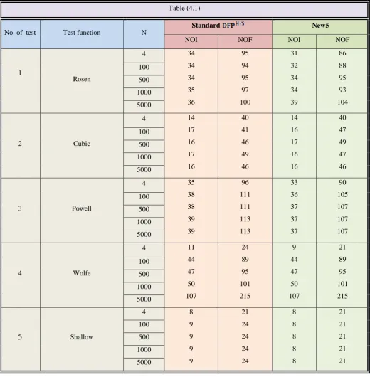
This section is devoted to test the implement of the new method. We compare the new update of DFP (New5) and standard . The comparative tests involve well known nonlinear problems (classical test function) with different function all programs are written in FORTRAN 95 language and for all cases the stopping condition

(8)

Comparative Performance of Standard and New5

Table (4.1)

No. of test Test function N

Standard New5

NOI NOF NOI NOF

1

Rosen

4 34

34 34 35 36 95 94 95 97 100 31 32 34 34 39 86 88 95 93 104 100 500 1000 5000

2 Cubic

4 14

17 16 17 16 40 41 46 49 46 14 16 17 16 16 40 47 49 47 46 100 500 1000 5000

3 Powell

4 35

38 38 39 39 96 111 111 113 113 33 36 37 37 37 90 105 107 107 107 100 500 1000 5000

4 Wolfe

4 11

44 47 50 107 24 89 95 101 215 9 44 47 50 107 21 89 95 101 215 100 500 1000 5000

5

Shallow

4 8

(9)

No. of test Test function N

Standard New5

NOI NOF NOI NOF

6

Wood

4 20

23 23 23 23 50 57 57 57 57 20 22 22 22 22 50 54 54 54 54 100 500 1000 5000

7 Non-diagonal

4 27

53 49 49 49 74 128 118 119 119 26 46 49 49 49 72 112 118 119 119 100 500 1000 5000

8 OSP

4 8

56 104 125 297 45 227 334 389 1028 8 48 104 124 297 45 185 338 388 1028 100 500 1000 5000

9 Mile

4 66

86 94 100 112 300 411 454 469 575 29 39 49 57 65 124 183 254 310 369 100 500 1000 5000

10

Beal

4 11

12 12 12 12 29 31 31 31 31 9 10 10 10 10 22 26 26 26 26 100 500 1000 5000

11

G-centeral

4 34

39 49 54 71 237 295 423 479 682 23 29 30 30 31 149 228 241 241 255 100 500 1000 5000

(10)

Comparing the Rate of Improvement between the new algorithm (New5) and the Standard Algorithm of

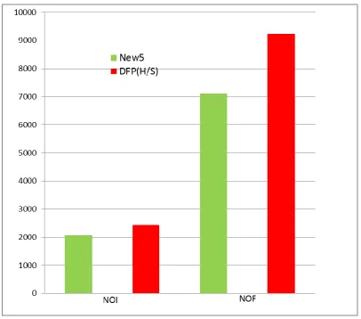
Table (4.3) shows the rate of improvement in the new algorithm (New5) with the standard algorithm (DFP), The numerical results of the new algorithm is better than the standard algorithm, As we notice that (NOI), (NOF) of the standard algorithm are about 100%, That means the new algorithm has improvement on standard algorithm prorate (15.2994%) in (NOI) and prorate (22.9593%) in (NOF), In general the new algorithm (New5) has been improved prorate (19.1294%) compared with standard algorithm (DFP).

Figure (4.1) shows the comparison between new algorithm (New5) and the standard algorithm (DFP) according to the total number of iterations (NOI) and the total number of functions (NOF).

5. CONCLUSION

(11)

References

[1]. A. Abashar, M. Mamat, M. Rivaie and I. Mohd, Global Convergence Properties of a New Class of Conjugate Gradient Method for Unconstrained Optimization, International Journal of Mathematical Analysis, 8 (2014), 3307-3319.

[2]. AL - Bayati, A.Y. and AL-Assady, N.H.,Conjugate gradient method,Technical Research , 1 (1986), school of computer studies, Leeds University.

[3]. E. Polak and G. Ribiere, Note sur la convergence de directionsconjugees, Rev. Francaise Informat Recherche Operationelle. 3(16) (1969), pp. 35-43.

[4]. J.E. Dennis and J.J. Mor6, "Quasi-Newton methods, motivation and theory," SIAM Review 19 a.(1977) 46-89.

[5]. J.E. Dennis and R.B. Schnabel, Numerical Methods for Unconstrained Optimization and Nonlinear a.Equations (Prentice-Hall, Englewood Cliffs, NJ, 1983).

[6]. M.R. Hestenes and E. Steifel, Method of conjugate gradient for solving linear equations, J. Res. Nat. Bur. Stand. 49 (1952), pp. 409-436.

[7]. M. Rivaie, A. Abashar, M. Mamat and I. Mohd, The Convergence Properties of a New Type of Conjugate Gradient Methods, Applied Mathematical Sciences, 8 (2014),33-44.

[8]. R. Fletcher, and C. Reeves, Function minimization by conjugate gradients, Comput. J. 7(1964), pp. 149-154.

[9]. R. Fletcher, Practical method of optimization, vol 1, unconstrained a.optimization, John Wiley & Sons, New York, 1987.

[10]. R. Fletcher, Practical Methods of Optimization: Unconstrained Optimization (Wiley, Chichester, 1980). [11]. P.E. Gill, W. Murray and M.H. Wright, Practical Optimization (Academic Press, New York, 1981). [12]. W.W. Hager, H. Zhang, A new conjugate gradient method with guaranteed descent and an efficient line

search, SIAM Journal on Optimization,16 (2005) 170–192

[13]. Y. H. Dai and Y. Yuan, A note on the nonlinear conjugate gradient method, J. Compt. Appl. Math., 18(2002), 575-582.