On Classification of Sleep Mechanism EEG Data
Pei Ling Lai1, Alfred Inselberg2
1Department of Electronics Engineering
Southern Taiwan University of Science and Technology Tainan, Taiwan, R.O.C.
2School of Mathematical Sciences Tel Aviv University, Tel Aviv, Israel
[email protected], [email protected]
ABSTRACT: We utilize a recent form of the Nested Cavities (abbr. NC) classifier [1] from which a powerful new classification approach emerged. In this application there are many outliers in the datasets [5] which judiciously removed. Further, working on the classification of Stage 3 we found wide dispersal in the data. After considerable experimentation we concluded that, between Stage2 and Stage3 some of the data is misclassified. By including some of the Stage2 data with values very close to those of Stage3 and forming a New-Stage 3 ALL nine of the measured variables have tight value ranges and the whole data set visually appears as a well-defined cluster. In turn, accurate classification rules are obtained which had not been possible for the original partition into stages. These findings are explained, motivated and analyzed here.
Keywords: Classification, Visualization, Parallel Coordinates, EEG Dataset
Received: 9 May 2013, Revised 15 June 2013, Accepted 22 June 2013
© 2013 DLINE. All rights reserved
1. Introduction
Classification is a basic task in data mining and pattern recognition [2]. From insight gained the NC classifier [3] a new step emerges significantly improving the classification. When the classifier either fails to converge or the rule is either very complex or inaccurate, the NC classifier discovers the dataset’s structure partitioning it into distinct subcategories which, in turn, can be more simply and accurately classified [1].
2. Classification Algorithm
With parallel coordinates (abbr. ||-coords) [4], a dataset P with N variables is transformed into a set of points in N dimensional space. In this setting, the designated subset S can be described by means of a hyper surface which encloses just the points of S. The description of such a hypersurface provides a rule for identifying, within an acceptable error, the elements of S. The use of Parallel Coordinates also enables visualization of the rule.
Figure 1. Construction of enclosure for the Nested Cavities algorithm
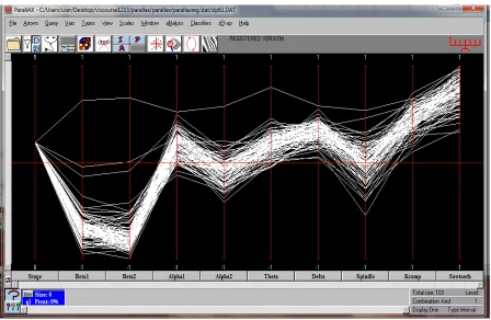
Figure 2. Slp61 dataset-Original stage 3 with 103 data entries, note outliers S1
S2
S3
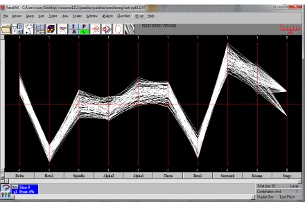
Figure 3. After cropping outliers there are 70 data entries
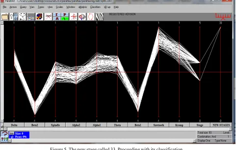
Figure 5. The new stage called 33. Proceeding with its classification
The first “wrapping” S1 is the convex hull of the points of S which also includes some points of P”S. The second wrapping S2 is the convex hull of these points and it includes some points of S which are enclosed with the third wrapping S3. To simplify the wrappings are shown as convex hulls rather than as approximations. Here the selected set is
S = (S1 − S2) ∪ (S3 − S4) where S4 = /0.
At first the algorithm determines a tight upper bound for the dimension R of S. For example, P may be a 3-dimensional set of points but all point of S may be on a plane; in which case S has dimension 2. Once R is determined R variables out of the N are chosen and ordered according to their predictive value and the construction process, schematically shown in Figure 1, operates only on these R selected variables.
The algorithm decomposes P into nested subsets, hence the name Nested Cavities (abbr. NC) for the classifier. The nested subsets are disjoint so they are partitions of P. Basically, the “wrapping” algorithm produces a convex-hull approximation; the technical details are not needed here. The efficiency of the version implemented here is due to the use of the R-coords representations of N-dimensional objects [4] applied in the description of the resulting hypersurface. It can and does happen that the process does not converge when P does not contain sufficient information to characterize S. It may also happen that S is so “porous” (i.e. sponge-like) that an inordinate number of iterations are required. The results (precision of rule) obtained by the NC classifier applied to bench-mark datasets were the most accurate when compared to those obtained by 22 other well-known classifiers (see [3]).The overall computational complexity is O(N2 | P |) where N is the number of variables and |P | is the number of points in P.
3. Simulation
3.1 Dataset
The raw EEG data were taken from the Physionet (MITBIH) Polysomnographic database. The subjects are male with an average age of 24-42 years. The data is taken with a sampling rate of 250 Hz and ADC resolution of 12 bits. While traditional EEG channels for sleep recording are placed either at C3-A2 or C4-A1 according to the 10-20 system for placement of EEG electrodes on the scalp [2-3]. The EEG recordings were taken from channels C3-O1, C4-A1 and O2-A1. The data are first converted from the .mat There are many outliers in the datasets which we decided to judiciously remove. The Slp61 dataset-Original stage 3 has 103 data entries, note outliers in Figure 2. We then cropped outliers so that there are 67 data entries Figure 3. Further, working on the classification of Stage 3 we found wide dispersal in the data. After considerable experimentation we e concluded that between Stage2 and Stage3 some of the data has have been misclassified.
3.2 Data Preprocessing
The single sided scaled amplitude spectrum of a real-valued time domain signal is computed for each harmonic parameter. The EEG is first filtered with a level 5 Butterworth high pass filter with cut-off frequencies between 0.5-30 Hz and then by a band stop filter on the 50-60Hz frequencies. The signal is further filtered using the Lab VIEW Wavelet De-noise. It performs noise reduction for 1D signals by using the discrete wavelet transform (DWT) or un-decimated wavelet transform (UWT). The transform used for the system is DWT using db04 wavelet with 7 levels and soft threshold.
3.3 Patitioning into sub- categoris
The EEG sleep dataset from [5] has been a real classification challenge. It has 9 variables, 760 observations in average and 5 stages consisting of wake (stage 0), light sleep (stage 1, 2), slow wave sleep (stages 3 and 4) and paradoxical sleep also known as the REM sleep [6]. The NC classifier was applied to the 11 patients (slp03, slp04, slp14, slp16, slp45, slp 48, slp59, slp60, slp61, slp66 and slp67) EEG datasets. We found stage 3 of patient 61 is the most informative dataset.
3.4 Forming a New-Stage
We then form a New-Stage 3 ALL nine of the measured variables have tight value ranges and the whole data set visually appears as a well-defined cluster. In turn, accurate classification rules are obtained which had not been possible for the original partition into stages.
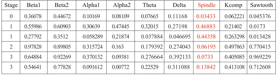
0 0.36078 0.44672 0.10169 0.08109 0.07665 0.11168 0.03433 0.062221 0.045376 1 0.55986 0.60903 0.30639 0.47445 0.32015 0.27198 0.46883 0.21402 0.0173 1 0.27792 0.3512 0.058289 0.21874 0.037884 0.046695 0.44358 0.263298 0.013428 2 0.97828 0.89805 0.315724 0.163 0.179392 0.274043 0.06195 0.497863 0.770415 3 0.64884 0.92269 0.370132 0.09381 0.276664 0.392133 0.0733 0.405085 0.969229 3 0.54641 0.77828 0.091612 0.00772 0.22529 0.311088 0.13842 0.413108 0.712608
Stage Beta1 Beta2 Alpha1 Alpha2 Theta Delta Spindle Kcomp Sawtooth
Table 1. Dataset Sample 7. Conclusion
Research on the automation of sleep stage classification, particularly single channel EEG, has been a challenge for many years. Our findings show that there are many outliers in the Physionet (MITBIH) Polysomnographic database which, we discovered after considerable experimentation, have been misclassified. This data is identified and new Stage 3 sets are formed whose classification reveals narrow range values of the measured waives providing a much clearer understanding of the sleep mechanism dynamics.
8. Acknowledhements
We are grateful to Aaron Raymond See and Prof. Shih Chung Chen for pointing out the Physionet (MITBIH) Polysomnographic database used here.
References
[1] Lai Jin Liang Yang, P. L., Inselberg, A. (2012). Geometric Divide and Conquer Classification for High-Dimensional Data, In: Proc. DATA, Rome: 79-82.
[2] Fayad, G., Piatesky-Shapiro, G., Smyth, P., Uthurusamy, R. Advances in Knowledge Discovery and Data Mining. AAAI/MIT Press.
[3] Inselberg, A., Avidan, T. (2000). Classification and Visualization for High-Dimensional Data, In: Proc. KDD, 370-4. ACM, New York.
[4] Inselberg, A. (1999). Parallel Coordinates: VISUAL Multidimensional Geometry and its Applications, Springer.
[5] Oropesa, E., Cycon, H. L., Jobert, M. Sleep Stage Classification using Wavelet Transform and Neural Network, International Computer Science Inst.
[6] Rechtschaffen, A., Kales, A. (1968). A Manual of Standardized Terminology, Techniques and Scoring System for Sleep Stages of Human Subjects, Brain Infor. Inst. UCLA.
[7] McBride, H. L., Peterson, G. L. (2004). Blind Data Classification Using Hyper-Dimensional Convex Polytopes, Flairs Conf. AAAI.
schematic in Figure 7 clarifies the partition.