The Thirty-Third AAAI Conference on Artificial Intelligence (AAAI-19)
A Theoretically Guaranteed Deep Optimization
Framework for Robust Compressive Sensing MRI
Risheng Liu,
1,2,∗Yuxi Zhang,
1,2Shichao Cheng,
2,3Xin Fan,
1,2Zhongxuan Luo
1,2,3,41DUT-RU International School of Information Science & Engineering, Dalian University of Technology, Dalian, China 2Key Laboratory for Ubiquitous Network and Service Software of Liaoning Province, Dalian, China
3School of Mathematical Science, Dalian University of Technology, Dalian, China 4Institute of Artificial Intelligence, Guilin University of Electronic Technology, Dalian, China
{rsliu, xin.fan, zxluo}@dlut.edu.cn, [email protected], [email protected]
Abstract
Magnetic Resonance Imaging (MRI) is one of the most dy-namic and safe imaging techniques available for clinical ap-plications. However, the rather slow speed of MRI acqui-sitions limits the patient throughput and potential indica-tions. Compressive Sensing (CS) has proven to be an effi-cient technique for accelerating MRI acquisition. The most widely used CS-MRI model, founded on the premise of re-constructing an image from an incompletely filled k-space, leads to an ill-posed inverse problem. In the past years, lots of efforts have been made to efficiently optimize the CS-MRI model. Inspired by deep learning techniques, some prelimi-nary works have tried to incorporate deep architectures into CS-MRI process. Unfortunately, the convergence issues (due to the experience-based networks) and the robustness (i.e., lack real-world noise modeling) of these deeply trained opti-mization methods are still missing. In this work, we develop a new paradigm to integrate designed numerical solvers and the data-driven architectures for CS-MRI. By introducing an optimal condition checking mechanism, we can successfully prove the convergence of our established deep CS-MRI op-timization scheme. Furthermore, we explicitly formulate the Rician noise distributions within our framework and obtain an extended CS-MRI network to handle the real-world nosies in the MRI process. Extensive experimental results verify that the proposed paradigm outperforms the existing state-of-the-art techniques both in reconstruction accuracy and efficiency as well as robustness to noises in real scene.
Introduction
Magnetic Resonance Imaging (MRI) is widely utilized in clinical applications because of its none-invasive property and excellent capability in revealing both functional and anatomical information. However, one of the main draw-backs is the inherently slow acquisition speed of MRI in k-space (i.e., Fourier k-space), due to the limitation of hardwares (Lustig et al. 2008). Compressive sensing MRI (CS-MRI) is a commonly used technique allowing fast acquisition at data sampling rate much lower than Nyquist rate without deteri-orating the image quality.
In the process of MR data acquisition, the sparse k-space dataycan be approximated as the following discretized
lin-∗
Corresponding Author.
Copyright c2019, Association for the Advancement of Artificial Intelligence (www.aaai.org). All rights reserved.
ear system (Eksioglu 2016):
y=PFx+n, (1)
wherex∈RN is the desired MR image to be reconstructed from observationy∈CM(M < N),Fis the Fourier trans-form,P ∈ RM×N denotes the under-sampling operation, andn∈CM represents the acquisition noises. It is easy to find that estimatingxfrom Eq. (1) is actually ill-posed, due to the singularity ofPF. Thus the main challenge for CS-MRI lies in defining proper regularizations and proposing corresponding nonlinear optimization or iterative algorithm for the inverse problem. According to CS theory, the most typical CS-MRI reconstruction techniques attempt to opti-mize the following nonsmooth regularized model:
α∈arg min
α
1
2kPFAα−yk
2
2+λkαkp, (2) whereαdenotes the sparse code ofx, corresponding to the wavelet basis (denoted asA, so we actually havex=Aα) of a given inverse wavelet transform (usually implemented by DCT or DWT) and λ indicates the trade-off parame-ter. In this work, we consider the `p regularization with
p∈(0,1), thus actually need to address a challenging non-convex sparse optimization task.
Related Works
In a conventional way, some effects are in exploring the sparse regularization in specific transform domain (Qu et al. 2012; Lustig, Donoho, and Pauly 2007; Gho et al. 2010). In addition, algorithms based on the nonlocal processing paradigm aim to construct a better sparsity transform, (Qu et al. 2014; Eksioglu 2016). Some dictionary learning based methods focus on training a dictionary from reference im-ages in the related subspace (Ravishankar and Bresler 2011; Babacan et al. 2011; Zhan et al. 2016). These model-based CS-MRI methods give satisfying performances in de-tails restoration benefiting from the model based data prior. While most of them are based on a sparsity introducing`1
norm or`0norm, which have weaker abilities to describe the
Recently, some preliminary studies on deep learning based CS-MRI have attracted great attentions (Wang et al. 2016; Lee, Yoo, and Ye 2017; Schlemper et al. 2018). At the expense of sacrificing principled information, such tech-niques benefit an extremely fast feed-forward process with the aid of deep architecture, but are not as flexible as the model based ones to handle various distributions of data.
To absorb the advantages of principled knowledge and data-driven prior, techniques are proposed integrating the deep architecture into an iterative optimization process (Liu et al. 2017; 2018a; 2018c; 2018b). By introducing learnable architectures into the Alternating Direction Method of Mul-tipliers (ADMM) iterations, they proposed an ADMM-Net to address the CS-MRI problem. In (Diamond et al. 2017) unrolled Optimization with Deep Priors (ODP) is proposed to integrate CNN priors into optimization process. It has been demonstrated that these deep priors can significantly improve the reconstruction accuracy. But unfortunately, due to their naive unrolling schemes (i.e., directly replace iter-ations by architectures), the convergence of these deep op-timization based CS-MRI methods cannot be theoretically guaranteed. Even worse, no mechanism is proposed to con-trol the errors generated by nested structures. Thus these methods may completely failed if improper architectures are utilized during iterations.
Except for the aforementioned problems, one concern but yet remain unsolved issue is the noise in MR images under real scene. During the practical acquisition of MR data, both real and imaginary parts of the complex data in k-space may be corrupted with uncorrelated zero-mean Gaussian noise with equal variance (Rajan et al. 2012). Thus the actual ac-quired magnitude MR imagexnis given as follows:
xn=
q
(xc+n1)2+n22, (3)
where xc denotes the noise-free signal intensity, and n1,n2 ∼ N(0, σ2) represent the uncorrelated real and
imaginary components of Gaussian noise, respectively. No-tice that the noise in magnitude MR image xn no longer follows the Gaussian distribution, but a Rician one.
Respectable effects for removing Rician noise from MR data have been made in several ways (Wiest-Daessl´e et al. 2008; Manj´on et al. 2010; Chen and Zeng 2015; Liu and Zhao 2016), but rather few studies on CS-MRI take into account the presence of actual noise in MR images. Ei-ther these CS-MRI methods consider only noiseless MR im-ages or treat the noise as a Gaussian one (Sun et al. 2016; Yang et al. 2018a). To the best of our knowledge, to date this matter has not been well solved in real sense.
Contributions
As discussed above, one of the most important limitations of existing deep optimization based CS-MRI methods (e.g., (Sun et al. 2016) and (Diamond et al. 2017)) is the lack of theoretical investigations. To address the aforementioned issues, in this paper, we propose a new deep algorithmic framework to optimize the CS-MRI problem in Eq. (2). Specifically, by integrating domain knowledge of the task and learning-based architectures, as well as checking the op-timal conditions, we can strictly prove the convergence of
our generated deep propagations. Moreover, due to the com-plex noise distributions (i.e., Rician), it is still challenging to directly apply existing CS-MRI methods to tasks in real-world scenarios. Thanks to the flexibility of our paradigm, we further extend the propagation framework to adaptively and iteratively remove Rician noise to guarantee the robust-ness of the MRI process. Our contributions can be summa-rized as follows:
• To our best knowledge, this is the first work that could establish theoretically convergent deep optimization algo-rithms to efficiently solve the nonconvex and nonsmooth CS-MRI model in Eq. (2). Thanks to the automatic check-ing and feedback mechanism (based on first-order opti-mality conditions), we can successfully reject improper nested architectures, thus will always propagate toward our desired solutions.
• To address the robustness issues in existing CS-MRI ap-proaches, we also develop an extended deep propagation scheme to simultaneously recover the latent MR images and remove the Rician nosies for real-world MRI process. • Extensive experimental results on real-world benchmarks demonstrate the superiority of the proposed paradigm against state-of-the-art techniques in both reconstruction accuracy and efficiency, as well as the robustness to com-plex noise pollution.
Our Paradigm for CS-MRI
In this section, we design a theoretically converged deep model to unify various of fundamental factors which affect the performance of CS-MRI. Different from most existing deep approaches, all of the fidelity knowledge, data-driven architecture, manual prior and optimality condition are com-prehensively taken into consideration in our deep frame-work. Meanwhile, the theoretical convergence is guaran-teed by our optimal checking mechanism. Inspired by recent studies (Liu et al. 2017; 2018a; Yang et al. 2018b), proximal gradient algorithm is utilized in this work to achieve an effi-cient optimization.
Fidelity Module:Fidelity plays an important role in reveal-ing the intrinsic genesis of problem, which is commonly adopted in traditional hand-crafted approaches. Actually, by given a reason manner to solve the fidelity term (i.e.,
1
2kPFAα−yk
2
2in Eq. (2)), we can generate a rough
restruction. Rather than introducing additional complex con-strains, here we just integrate the current restorationαkwith the fidelity and consider the following subproblem:
uk+1= arg min
u
1
2kPFAu−yk
2 2+
ρ
2ku−α
kk2
2, (4)
where ρ denotes the weight parameter and A contains a wavelet basis corresponding to an inverse wavelet transform. Eq. (4) provides a balance of αk and fidelity term, thus an additional benefit is that the restorationαk can be cor-rected by the fidelity whileαkis out of the desired descent direction. Benefiting from the continuity of the function in Eq. (4), a closed solution can be derived through Eq. (5):
uk+1=F αk;ρ=ATFT PTP+ρI−1 PTy+ρFAαk.
Data-driven Module:Inspired by the deep methods which can effectively simulate the data distribution by training nu-merous paired input and output. A learning based module with deep architecture is taken into account to utilize the implicit data based distribution. Notice that previous work has demonstrated an insufficient sparsity representation in the pre-defined sparse transform will introduce artifacts dur-ing the process (Knoll et al. 2011; Liang et al. 2011). Fur-thermore, the previous fidelity based optimization may also bring in artifacts. Thus a residual learning network with shortcut is adopted as a denoiser. We define this module as
vk+1=N uk+1;ϑk+1, (6)
whereϑk+1 is the parameter of network in thek-th stage.
Notice that here both the input and output are in image do-main. Thus the transformation between image and sparse code is incorporated into the network. In the experiments section, we will give a concrete example of the choice for such CNN denoiser.
Optimal Condition Module: Two major arguments
aris-ing with data-driven module are: 1) whether the direction generated by deep architecture can satisfy the convergence analysis (i.e., updating along a descent direction); 2) losing the empirical prior, whether the output of network trends to search a desired optimality solution.
To clarify above doubts, a checking mechanism based on first-order optimal condition is proposed to indicate whether the updating by deep architecture is satisfied and which vari-able should be adopted in the next iterations. First, we intro-duce a proximal gradient with momentum term to connect the output of data-driven network with the first-order opti-mal condition of a constructed minimization energy. Here, we define the momentum proximal gradient1as
βk+1∈proxη
1λk·kpv k+1−η
1∇f vk+1
+ρvk+1−αk ,
(7) whereη1is the step-size andf denotes the fidelity term in
Eq. (2). Then we establish feedback mechanism by consid-ering the first-order optimal condition of Eq. (7) as
kvk+1−βk+1k ≤εkkαk−βk+1k. (8)
Here,εkis a positive constant to reveal the tolerance scale of the distance between current solutionβk+1and the last up-datingαkat thek-th stage. Finally,αkis also re-considered when Eq. (8) is not satisfied. Thus, our checking module can be simplified as
wk+1=C(vk+1,αk) =
βk+1 Eq.(8)
αk otherwise. (9)
Prior Module:Manual sparse prior is a widely used com-ponent to constrain the desired solution in traditional opti-mization. It also naturally describes the distribution of MRI. Thus, it makes sense to introduce the sparsity for a better CS-MRI restoration. We append a prior module after check-ing mechanism to pick the penalty termλkvkpin Eq. (2) up again. Considering the nonconvexity of`p-norm regulariza-tion, we solve it by a step of proximal gradient as following:
1
proxηλk·kp(v) = arg minxλkxkp+
1 2kx−vk
2
.
Algorithm 1The proposed framework
Require: x0,P,F,y,and some necessary parameters.
Ensure: Reconstructed MR imagex.
1: while not convergeddo
2: uk+1=F αk;ρ ,
3: vk+1=N uk+1;ϑk+1 ,
4: wk+1=C vk+1,αk ,
5: αk+1=P wk+1;η2
,
6: end while
7: x=Aα∗.
αk+1=P wk+1;η2
∈proxη2λk·kp wk+1−η2∇f wk+1
,
(10) whereη2 is the step-size. In this way, we can enhance the
effect of original model and naturally correct over-smooth and preserve more details.
Considering all the aforementioned settlements, we can reconstruct the fully-sampled MR data by iteratively solving corresponding subproblems as showed in Alg. 1. We restore the clear MRI by the final estimationα∗.
Theoretical Investigations
Different from existing deep optimization strategies (Sun et al. 2016; Diamond et al. 2017), which discard the conver-gence guarantee in iterations and almost rely on the distribu-tion of training data. Our scheme not only merges the tradi-tional designed model optimization about fidelity and sparse prior, but also introduces the learnable network architecture into our deep optimization framework. Furthermore, we also provide an effective mechanism to discriminate whether the output of network in current iteration is a desired descent direction. In the following, we will analyze the strict conver-gence behavior of our method.
To simplify the following derivations, we first rewrite the function in Eq. (2) as
Φ(α) = 1
2kPFAα−yk 2
2+λkαkp.
Furthermore, we also state some properties aboutΦwhich are helpful for the convergence analysis as following2:
(1) 12kPFAα−yk2
2is proper and Lipschitz smooth;
(2)λkαkpis proper and lower semi-continuous; (3)Φ(α)satisfies KŁ property and is coercive.
Then some important Propositions are given to illustrate the convergence performance of our approach.
Proposition 1 Let αk
k∈N and
βk
k∈N be the se-quences generated by Alg. 1. Suppose that the error con-ditionkvk+1−αkk ≤ εkkβk+1−αkkin ouricheckis
satisfied. Then there exists a sequence{Ck}k∈Nsuch that
Φ(βk+1)≤Φ(αk)−Ckkβk+1−αkk2, (11)
whereCk= 1/2η
1−Lf/2−(Lf+|ρ−1/η1|)k >0and
Lf is the Lipschitz coefficient of∇f.
2
Proposition 2 Ifη2 < 1/Lf, let
αk k∈
Nand
wk k∈
N be the sequences generated by a proximal operator in Alg. 1. Then we have
Φ(αk+1)≤Φ(wk+1)−(1/(2η2)−Lf/2)kαk+1−wk+1k2. (12)
Remark 1 Actually, the inequality in Propositions 1 and 2 provide a descent sequenceΦ(αk)by illustrating the
rela-tionship ofΦ(αk)andΦ(wk)as
−∞<Φ(αk+1)≤Φ(wk)≤Φ(αk)≤Φ(α0).
Thus, the operatorCis a key criterion to check whether the output of our designed network propagates along a descent direction. Moreover, it also ingeniously builds a bridge to connect the adjacent iterationΦ(αk)andΦ(αk+1).
Theorem 1 Suppose thatαk
k∈N be a sequence gener-ated by Alg. 1. The following assertions hold.
• The square summable of sequenceαk+1−wk+1 k∈
N is bounded, i.e.,P∞
k=1kα
k+1−wk+1k2<∞.
• The sequenceαk
k∈Nconverges to a critical pointα ∗
ofΦ.
Remark 2 The second assertion in Theorem 1 implies that
αk
k∈Nis a Cauchy sequence, thus it globally converges to the critical point ofΦ.
Real-world CS-MRI with Rician Noises
It is worth noting that robustness is important in CS-MRI. Unfortunately, most strategies only consider the scenario without noise thus they usually fail on real-world cases. To enable our method handle the task of CS-MRI with Rician noise, we extend our CS-MRI model in Eq. (2) as:min
x 1
2kPFz−yk
2
2+λ1kA>1xkp+λ2kA>2zkp
s.t. z=p(x+n1)2+n22,
(13)
wherex,y,n1, andn2denotes the fully sampled clear MR
image, sparse k-space data, the uncorrelated Gaussian noise in real and imaginary component respectively.A>1 andA>2 are inverse of the wavelet transformA1andA2respectively. Optimization Strategy:We can rewrite Eq. (13) by splitting it as the following subproblems:
zk+1= arg min z
1
2kPFz−yk
2
2+λ1kA>1zkp
+ρ1 2kz−
p
(xk+n
1)2+n22k22,
(14a)
xk+1= arg min x
1 2k
p
(x+n1)2+n22−zk+1k22
+λ2kA>2xkp,
(14b)
where ρ1 is the penalty parameter. Thus, we can
subse-quently tackle each of them with the iterations in Alg. 1 to solvezk+1andxk+1respectively.
For the subproblem Eq. (14a), which aims to reconstruct the fully sampled noisy MR image from k-space observa-tiony, we can optimize it similarly with the aforementioned CS-MRI problem by assuming the fidelity including both CS and noise (i.,e., two square term), respectively. In terms of the second subproblem Eq. (14b), the solution is a clear
0 50 100 150 200
Iteration -10 -9 -8 -7 -6 -5 -4 -3 -2
0 50 100 150 200
Iteration 25 26 27 28 29 30 31
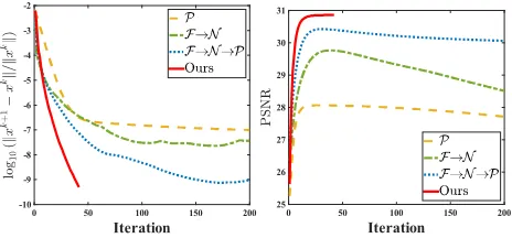
Figure 1: Quantitative results of four optimization models.
P F→N F→N→P Ours
Figure 2: Qualitative results of four optimization models.
Cartesian Mask Radial Mask Gaussian Mask 20 24 28 32 36 40 PS N R ZF TV SIDWT PBDW PANO FDLCP ADMM BM3D-MRI Ours
Figure 3: Comparisons using various sampling patterns.
10 20 30 40 50
Sampling Ratio 0.04 0.08 0.12 0.16 0.2 0.24 R L N E TV SIDWT PBDW PANO FDLCP ADMM BM3D-MRI Ours
10 20 30 40 50
Sampling Ratio 0 0.1 0.2 0.3 0.4 0.5 M SE TV SIDWT PBDW PANO FDLCP ADMM BM3D-MRI Ours
Figure 4: Comparisons under different sampling ratios.
image. We cannot straightly obtain the closed-form solution due to the quadratic term(x+n1)2. Thus, a learnable
strat-egy is adopted to restore a rough MRI in fidelity module.
Learnable Architecture for Rician Noise Removal: It is
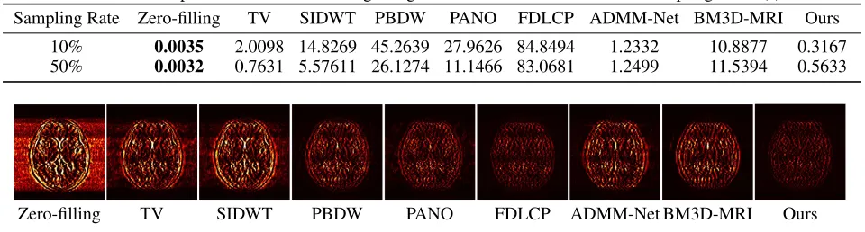
net-Table 1: Comparison of time consuming using Radial mask with two different sampling ratios (s).
Sampling Rate Zero-filling TV SIDWT PBDW PANO FDLCP ADMM-Net BM3D-MRI Ours
10% 0.0035 2.0098 14.8269 45.2639 27.9626 84.8494 1.2332 10.8877 0.3167
50% 0.0032 0.7631 5.57611 26.1274 11.1466 83.0681 1.2499 11.5394 0.5633
Zero-filling TV SIDWT PBDW PANO FDLCP ADMM-Net BM3D-MRI Ours
Figure 5: Visualization of the reconstruction error using Cartesian mask with 30% sampling rate.
Ground Truth (PSNR) Zero-filling (22.33) TV (25.22) SIDWT (25.10) PBDW (27.39)
PANO (28.77) FDLCP (29.78) ADMM-Net (27.91) BM3D-MRI (29.35) Ours (30.48)
Figure 6: Qualitative comparison onT1-weighted brain MRI data using Gaussian mask with 10% sample rate.
work to learn(xc+n1)2fromx2n(i.e.,(xc+n1)2+n22). To
release the square operator underxc, we train the other one by feedingp(xc+n1)2andxcas input and output.
Experimental Results
In this section, we first explore the roles of each module and theoretical results in our paradigm. To demonstrate the supe-riority of our method, we then compare it with some state-of-the-art techniques on both traditional and real-world CS-MRI. All experiments are executed on a PC with Intel(R) Gold 6154 CPU @ 3.00GHz 256 GB RAM and a NVIDIA TITAN Xp. Notice that we performp= 0.8in experiments.
CS-MRI Reconstruction
We first analyze the effects of modules and verify the theo-retical convergence by ablation experiments. Then we per-form comparisons on traditional CS-MRI in perspective of reconstruction accuracy, time consuming and robustness.
Ablation Analysis: First we compare four different
com-binations of modules in our framework. The first one is to reconstruct directly with the prior module to figure out the role of a manual prior, the second one is to integrate the data-driven module with the fidelity module to explore the effect of data based distribution, and the third choice is combina-tion of these three modules. Adding the optimal condicombina-tion
module, we get the entire paradigm as the last choice. For convenience, we refer them asP,F →N,F →N →P and
Oursrespectively. We apply these strategies onT1-weighted
data using Ridial sampling pattern with 20% sampling rate. The stopping criteria is set askxk+1−xkk/kxkk ≤1e−4. As shows in Fig. 1, at the first several iterations, the loss ofP is slightly larger than that ofF →N. Because the in-put is corrupted with severe artifacts, thus the role of data-driven module is significant at the first several steps. But as process goes on, repeated denoising operation in turn causes over-smoothing. While moduleP can make up for it by in-corporating model based knowledge. ThoughF → N → P can improve the performance, it cannot ideally converge to a desired solution. The solid line indicates the superiority ofOursover other choices in both convergence rate and re-construction accuracy. The execution time of P ,F → N, F → N → P andOurs is 4.4762s, 3.3240s, 6.2760s and 2.5225s, respectively. As expect, the proposed method pro-vides a much faster reconstruction process. Thus we can ver-ify that our framework has higher efficiency both in terms of theoretical convergence and practical execution time. The visualized results in Fig. 2 also verify that Ours has better performance than others.
Comparisons with Existing Methods:In this section, we
includ-Table 2: Comparison on different testing data using Cartesian mask at a sampling rate of 30%
MRI Data Zero-filling TV SIDWT PBDW PANO FDLCP ADMM-Net BM3D-MRI Ours
Chest 22.95 24.43 24.17 25.91 27.73 26.84 25.38 26.27 28.22
Cardiac 23.40 29.17 27.49 31.34 33.14 33.84 31.42 31.44 35.69
Renal 24.32 28.77 27.66 31.05 32.21 33.74 31.13 31.01 34.79
Ground Truth (PSNR) PANO (27.73) FDLCP (26.84) BM3D-MRI (26.27) Ours (28.22)
Figure 7: Qualitative comparisons on chest data using Cartesian mask with 30% sampling rate.
0.39 0.42 0.45 0.48 0.51 SSIM
20 20.9 21.8 22.7 23.6 24.5
PS
N
R
ZF TV SIDWT PBDW PANO FDLCP ADMM-Net BM3D-MRI Ours
0.28 0.31 0.34 0.37 0.4 SSIM
20 20.9 21.8 22.7 23.6 24.5
PS
N
R
ZF TV SIDWT PBDW PANO FDLCP ADMM-Net BM3D-MRI Ours
0.39 0.42 0.45 0.48 0.51 SSIM
20 20.9 21.8 22.7 23.6 24.5
PS
N
R
ZF TV SIDWT PBDW PANO FDLCP ADMM-Net BM3D-MRI Ours
0.28 0.31 0.34 0.37 0.4 SSIM
20 20.9 21.8 22.7 23.6 24.5
PS
N
R
ZF TV SIDWT PBDW PANO FDLCP ADMM-Net BM3D-MRI Ours
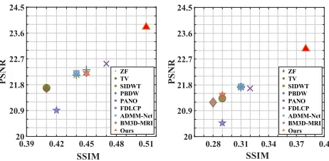
Figure 8: Comparison of robustness. Left and right subfig-ures represent the results ofT1-weighted andT2-weighted
data, respectively.
Noisy BM3D-MRI RiceOptVST Our Denoiser
Figure 9: Comparison between our denoiser (PSNR:31.72) and RiceOptVST (PSNR:30.34) for denoising.
ing Zero-filling (Bernstein, Fain, and Riederer 2001), TV (Lustig, Donoho, and Pauly 2007) and SIDWT (Baraniuk 2007), and five state-of-the-art like PBDW (Qu et al. 2012), PANO (Qu et al. 2014), FDLCP (Zhan et al. 2016), ADMM-Net (Sun et al. 2016) and BM3D-MRI (Eksioglu 2016). 25
T1-weighted MRI data and 25 T2-weighted MRI data are
randomly chosen from 50 subjects in IXI datasets3 as the testing data. In the experiment process, the parameterρin moduleFis set as 5 and the noise level of network in mod-uleN ranges from 3.0 to 50.0. Parameter L (η = 2/L),λ
and p in modulesC andP are set as 1.1, 0.00001 and 0.8, respectively. The number of total iterations is 50. As for the
3
http://brain-development.org/ixi-dataset/
parameters of comparative approaches, we adopt the most proper settings as suggested in their papers for fairness.
First, we test on 25 T1-weighted MRI data using three
different undersampling patterns with a fixed 10% sam-pling rate. Fig. 3 shows the quantitative results (PSNR). Our method performs best for all three cases and has stronger sta-bility compared with the second best method on variance. As for the effect of sampling ratios variation, we use radial mask under 10%, 30% and 50% sampling rates with evaluation of RLNE and MSE. Fig. 4 shows that our method has the low-est reconstruction error for all sampling rates. For more in-tuitive comparison, we illustrate the reconstruction error in term of pixels in Fig. 5. We also offer the qualitative com-parison in Fig. 6. Visualized results demonstrate our method has better performance in both artifacts removing and details restoration. Time consuming is also considered. We com-pare our method with others on the 25 T1-weighted data
us-ing Radial mask with 10% and 50% samplus-ing rate. Notice that ADMM-Net and ours are tested on GPU for the incor-poration of deep architecture. Tab. 1 shows that our method provides an efficient reconstruction process and comes to the fastest method among the state-of-the-art competitors.
To demonstrate the robustness of our approach, we first apply it on various MRI data including the chest, cardiac and renal (Yazdanpanah and Regentova 2017). In Tab. 2, Our proposed framework gives the highest PSNR for all of the tree types of MR images. Fig. 7 visualizes the correspond-ing results for chest data. we can see that our approach pre-vails over others in detail restoration at the junction of blood vessels as well as noise removal in the background. Actu-ally, our method has a stronger ability to handle slight noise because of the subprocess of learning based optimization with deep prior. To demonstrate that, we add Rician noise at level of 20 to 25 T1-weighted MRI and 25 T2-weighted
Table 3: Comparison between our framework and traditional CS-MRI methods followed by a denoiser.
MRI Data Denoiser Zero-filling TV SIDWT PBDW PANO FDLCP ADMM-Net BM3D-MRI Ours
T1-weighted Our DenoiserRiceOptVST 24.1124.62 25.5125.71 25.7825.94 26.6526.83 27.3027.08 25.5925.66 26.4926.36 27.3627.64 28.05
T2-weighted Our DenoiserRiceOptVST 25.4026.36 27.8328.20 28.3728.68 29.1329.46 29.6429.22 27.4427.55 29.4529.14 29.6730.34 30.77
Ground Truth (PSNR) FDLCP (25.72) ADMM-Net (26.29) BM3D-MRI (27.41) Ours (28.42)
Figure 10: Qualitative comparison between our framework and traditional CS-MRI methods.
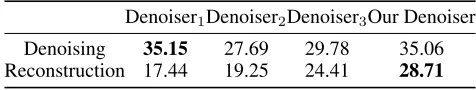
Table 4: Comparison between four types of CNN denoiser.
Denoiser1Denoiser2Denoiser3Our Denoiser
Denoising 35.15 27.69 29.78 35.06 Reconstruction 17.44 19.25 24.41 28.71
Real-world CS-MRI
We further explore the performance of our approach on real-world CS-MRI with Rician noise and the parametersρ1,λ1
andλ2 in Eq. (13a) and Eq. (13b) are set as 0.01, 1.0 and
1.0, respectively.
Rician Network Behavior:In the learnable architecture, the first stage is to get(xc+n1)2and the second stage is to
ob-tain the desired noise-free dataxcin Eq. (3). At the training stage, we generate Rician noisy input data withσ= 20 us-ing 500T1-weighted MR images randomly picked from the
MICCAI 2013 grand challenge dataset4.
To verify the effectiveness of our learnable Rician net-work, we offer some other possible ways to obtain the xc fromxnthrough deep learning.Denoiser1directly learns the
difference betweenxn andxc.Denoiser2learns the
Gaus-sian noise existing in the real and imaginary parts separately.
Denoiser3treats the Rician noise as a Gaussian one. For all
the four types of denoisers, we use the same network ar-chitecture as IRCNN (Zhang et al. 2017). Tab. 4 shows that
Denoiser1gives comparable performance in denoising, but
performs the worst for real-world CS-MRI. On the contrary, our learnable architecture gives a much better result than other methods. It is because the Rician noise is not additive noise. Directly estimation from the difference ofxcandxn may cause error especially when the noise in the background is large. We also compare with the classical Rician denoising technique RicieOptVST5 (Foi 2011) to evaluate our
learn-4
http://masiweb.vuse.vanderbilt.edu/workshop2013/index.php /Segmentation Challenge Details
5
http://www.cs.tut.fi/ foi/RiceOptVST/#ref software
able architecture. Fig. 9 shows our learnable architecture has a better performance in removing the noise on background, indicating that we can also take the learnable architecture to address pure Rician denoising issues.
Benchmark:We then compare our method with other
CS-MRI techniques on the task of CS-CS-MRI with noise. The
T1-weighted andT2-weighted MRI data in IXI dataset are
adopted as test benchmark. Since the compared methods don’t have mechanism to handle Rician noise, we separately assign a classical Rician noise remover RicieOptVST and our learnable architecture for them to execute the denois-ing after CS reconstruction. As shows in Tab. 3, our CS-MRI framework has superiority against others based on both
RicieOptVST and our network. Furthermore, the choice of taking our learnable architecture as the denoiser performs better than that of takingRiceOptVST and the last column shows that the proposed framework surpasses all the com-binations. In Fig. 10, we can have a more intuitive under-standing to the reconstruction comparison. More details are preserved in our framework than competitive approaches.
Conclusions
We propose a theoretically converged deep optimization framework to efficiently solve the nonconvex and nons-mooth CS-MRI model. Our framework can take advantage of fidelity, prior, data-driven architecture and optimal con-dition to guarantee the iterative variables converge to criti-cal point of the specific model. For real-world CS-MRI with Rician noise, a learning based architecture is proposed for Rician noise removal. Experiments demonstrate that the our framework is robust and superior than others.
Acknowledgments
References
Babacan, S. D.; Peng, X.; Wang, X.; Do, M. N.; and Liang, Z. 2011. Reference-guided sparsifying transform design for compressive sensing mri. InEMBC, 5718–5721. IEEE. Baraniuk, R. G. 2007. Compressive sensing [lecture notes].
IEEE SPM24(4):118–121.
Bernstein, M. A.; Fain, S. B.; and Riederer, S. J. 2001. Effect of windowing and zero-filled reconstruction of mri data on spatial resolution and acquisition strategy.JMRI14(3):270– 280.
Chen, L., and Zeng, T. 2015. A convex variational model for restoring blurred images with large rician noise. JMIV
53(1):92–111.
Diamond, S.; Sitzmann, V.; Heide, F.; and Wetzstein, G. 2017. Unrolled optimization with deep priors. arXiv preprint arXiv:1705.08041.
Eksioglu, E. M. 2016. Decoupled algorithm for mri recon-struction using nonlocal block matching model: Bm3d-mri.
JMIV56(3):430–440.
Foi, A. 2011. Noise estimation and removal in mr imaging: The variance-stabilization approach. InISBI, 1809–1814. Gho, S. M.; Nam, Y.; Zho, S. Y.; Kim, E. Y.; and Kim, D. H. 2010. Three dimension double inversion recovery gray mat-ter imaging using compressed sensing. JMRI28(10):1395– 1402.
Knoll, F.; Bredies, K.; Pock, T.; and Stollberger, R. 2011. Second order total generalized variation (tgv) for mri. Mag-netic Resonance in Medicine65(2):480–491.
Lee, D.; Yoo, J.; and Ye, J. C. 2017. Deep residual learning for compressed sensing mri. InISBI, 15–18.
Liang, D.; Wang, H.; Chang, Y.; and Ying, L. 2011. Sensitiv-ity encoding reconstruction with nonlocal total variation reg-ularization. Magnetic Resonance in Medicine65(5):1384– 1392.
Liu, J., and Zhao, Z. 2016. Variational approach to second-order damped hamiltonian systems with impulsive effects.
JNSA9(6):3459–3472.
Liu, R.; Cheng, S.; Liu, X.; Ma, L.; Fan, X.; and Luo, Z. 2017. A bridging framework for model optimization and deep propagation. InNIPS.
Liu, R.; Cheng, S.; He, Y.; Fan, X.; Lin, Z.; and Luo, Z. 2018a. On the convergence of learning-based iterative methods for nonconvex inverse problems. arXiv preprint arXiv:1808.05331.
Liu, R.; Fan, X.; Hou, M.; Jiang, Z.; Luo, Z.; and Zhang, L. 2018b. Learning aggregated transmission propagation net-works for haze removal and beyond. IEEE TNNLS(99):1– 14.
Liu, R.; Ma, L.; Wang, Y.; and Zhang, L. 2018c. Learning converged propagations with deep prior ensemble for image enhancement.IEEE TIP.
Liu, R.; Zhang, Y.; Cheng, S.; Fan, X.; and Luo, Z. 2018d. A theoretically guaranteed deep optimization frame-work for robust compressive sensing mri. arXiv preprint arXiv:1811.03782.
Lustig, M.; Donoho, D. L.; Santos, J. M.; and Pauly, J. M. 2008. Compressed sensing mri.IEEE SPM25(2):72–82. Lustig, M.; Donoho, D.; and Pauly, J. M. 2007. Sparse mri: The application of compressed sensing for rapid mr imaging.
Magnetic Resonance in Medicine58(6):1182–1195. Manj´on, J. V.; Coup´e, P.; Mart´ı-Bonmat´ı, L.; Collins, D. L.; and Robles, M. 2010. Adaptive non-local means denois-ing of mr images with spatially varydenois-ing noise levels. JMRI
31(1):192–203.
Qu, X.; Guo, D.; Ning, B.; Hou, Y.; Lin, Y.; Cai, S.; and Chen, Z. 2012. Undersampled mri reconstruction with patch-based directional wavelets. MRI30(7):964–977. Qu, X.; Hou, Y.; Lam, F.; Guo, D.; Zhong, J.; and Chen, Z. 2014. Magnetic resonance image reconstruction from undersampled measurements using a patch-based nonlocal operator.Medical Image Analysis18(6):843–856.
Rajan, J.; Van Audekerke, J.; Van der Linden, A.; Verhoye, M.; and Sijbers, J. 2012. An adaptive non local maximum likelihood estimation method for denoising magnetic reso-nance images. InISBI, 1136–1139. IEEE.
Ravishankar, S., and Bresler, Y. 2011. Mr image reconstruc-tion from highly undersampled k-space data by dicreconstruc-tionary learning.IEEE TMI30(5):1028.
Schlemper, J.; Caballero, J.; Hajnal, J. V.; Price, A. N.; and Rueckert, D. 2018. A deep cascade of convolutional neural networks for dynamic mr image reconstruction. IEEE TMI
37(2):491–503.
Sun, J.; Li, H.; Xu, Z.; et al. 2016. Deep admm-net for compressive sensing mri. InNIPS, 10–18.
Wang, S.; Su, Z.; Ying, L.; Peng, X.; Zhu, S.; Liang, F.; Feng, D.; and Liang, D. 2016. Accelerating magnetic reso-nance imaging via deep learning. InISBI, 514–517. Wiest-Daessl´e, N.; Prima, S.; Coup´e, P.; Morrissey, S. P.; and Barillot, C. 2008. Rician noise removal by non-local means filtering for low signal-to-noise ratio mri: applica-tions to dt-mri. InMICCAI, 171–179.
Yang, G.; Yu, S.; Dong, H.; Slabaugh, G.; Dragotti, P. L.; Ye, X.; Liu, F.; Arridge, S.; Keegan, J.; Guo, Y.; et al. 2018a. Dagan: Deep de-aliasing generative adversarial networks for fast compressed sensing mri reconstruction. IEEE TMI
37(6):1310–1321.
Yang, Z.; Xu, Q.; Cao, X.; and Huang, Q. 2018b. From com-mon to special: When multi-attribute learning meets person-alized opinions. InAAAI, 515–522.
Yazdanpanah, A. P., and Regentova, E. E. 2017. Com-pressed sensing magnetic resonance imaging based on shearlet sparsity and nonlocal total variation. JMI
4(2):026003.
Zhan, Z.; Cai, J.; Guo, D.; Liu, Y.; Chen, Z.; and Qu, X. 2016. Fast multiclass dictionaries learning with geometrical directions in mri reconstruction. IEEE TBME63(9):1850– 1861.