Approximate Profile Maximum Likelihood
Dmitri S. Pavlichin [email protected]
Department of Applied Physics Stanford University
Stanford, CA 94305, USA
Jiantao Jiao [email protected]
Department of Electrical Engineering and Computer Sciences University of California
Berkeley, CA 94720, USA
Tsachy Weissman [email protected]
Department of Electrical Engineering Stanford University
Stanford, CA 94305, USA
Editor:Sara van de Geer
Abstract
We propose an efficient algorithm for approximate computation of the profile maximum likelihood (PML), a variant of maximum likelihood maximizing the probability of observing a sufficient statistic rather than the empirical sample. The PML has appealing theoretical properties, but is difficult to compute exactly. Inspired by observations gleaned from ex-actly solvable cases, we look for an approximate PML solution, which, intuitively, clumps comparably frequent symbols into one symbol. This amounts to lower-bounding a certain matrix permanent by summing over a subgroup of the symmetric group rather than the whole group during the computation. We extensively experiment with the approximate solution, and the empirical performance of our approach is competitive and sometimes significantly better than state-of-the-art performances for various estimation problems. Keywords: Profile maximum likelihood, dynamic programming, sufficient statistic, par-tition of multi-partite numbers, integer parpar-tition
1. Introduction
The maximum likelihood principle, proposed by Ronald Fisher, has proved to be a powerful and versatile method used throughout nearly all scientific fields. However, it is still the source of considerable controversy in the statistics and machine learning community. Indeed, quoting Efron (Efron, 1982):
“The controversy centers on the relationship between decision theory and maximum likelihood. Beginning with the Neyman-Pearson lemma, decision theory has reshaped the theory and practice of hypothesis testing...”
Indeed, Wald’s statistical decision theory (Wald, 1950) provided a comprehensive frame-work for evaluating and proposing statistical procedures. The maximum likelihood ap-proach, which can be proved to be asymptotically efficient under mild conditions in the
c
H´ajek-Le Cam theory (Van der Vaart, 2000, Chap. 9), lacks a finite-sample justification. Indeed, as Le Cam (Le Cam, 1979) argued, even in the asymptotic regime the maximum likelihood approach may have weird behavior and is not always consistent.
The recent work (Acharya et al., 2017) provided an elegant justification of the maxi-mum likelihood approach which is intimately connected to decision theory. It was shown in (Acharya et al., 2017) that plugging-in the profile maximum likelihood (PML) distri-bution estimators into a variety of functionals achieves the optimal sample complexity in estimating those functionals, which the generic sequence maximum likelihood (SML) fails to achieve. We also refer the readers to (Anevski et al., 2017) for statistical properties of PML.
To compute the profile maximum likelihood estimator we must solve the following op-timization problem: givenn samples with empirical distribution ˆp= (ˆp1,pˆ2, . . .), maximize the probability to observe ˆp up to relabeling σpˆ,(ˆpσ(1),pˆσ(2), . . .) of the empirical distri-bution, where σ is some permutation. This amounts to computing the PML distribution
p∗:
p∗ = argmax p
X σ
Pp(σpˆ) = argmax
p X
σ
e−nD(σpˆ||p) (1)
where the max is over all discrete distributions p with a known support set size (we treat the unknown case later; it is similar), the sum is over all permutationsσ of the support set of distribution p, and whereD(·||·) is the Kullback-Leibler divergence.
The profile maximum likelihood estimator is computationally challenging to find – as can shown to be equivalent to optimizing a certain matrix permanent – and the best known algorithm has running time exponential in the support size of the unknown discrete distri-bution. Our main contributions are the following:
1. We present an efficiently computable approximation for the PML distribution. The approximation idea is motivated by observations for the exact PML for small alpha-bets, where the PML distribution tends to put symbols whose empirical counts are close (within O(√n)) into the same level set1. The idea is to lower bound the sum in (1) by summing over only the permutations that contribute “a lot” – namely the subgroup of permutations that only mix symbols within the level sets ofp. This leads to the objective function in the argmax below (a lower bound to the objective function in (1)) to define the approximate PML (APML) distribution ¯p∗:
¯
p∗= argmax p
e−nD( ˆp||p) Y
α∈A(p)
|α|!
(2)
where A(p) is the partition of the support set of p into the level sets α of p. The second factor of the objective function rewards clumping many symbols together into a few large level sets, while the first factor encourages similarity to the empirical distribution and dominates as the sample sizen→ ∞.
We present a dynamic programming approach to compute the approximate PML distribution ¯p∗. Compared with existing approximations to the PML (Orlitsky et al., 2004b; Vontobel, 2012), our algorithm has no tuning parameters, is deterministic, runs
in at most linear time in the sample size (usually computing the empirical histogram is the slowest part), and achieves state-of-the-art empirical performance in various estimation tasks that we detail below.
For the case of unknown support set size, we state the appropriate generalization of the PML distribution and its approximation. We modify our dynamic programming algorithm slightly to handle this case, preserving a linear worst-case runtime. It may happen that the PML and our approximate PML distributions have a discrete part with finite support and a “continuous part” in the terminology of (Orlitsky et al., 2004b); we are able to detect this case and find the discrete part of the approximate PML distribution and the probability mass of the continuous part.
2. Given the result in (Acharya et al., 2017) that plugging in the PML distribution into various functionals achieves the optimal sample complexity, we extensively experi-ment with the plug-in estimator using our APML distribution. We estimate entropy, R´enyi entropy, support set size, L1 distance to uniformity, and the sorted probabil-ity vector of a discrete distribution and compare with the state-of-the-art approaches with available code for estimating those functionals. We find that the performance of plugging in our APML distribution into those functionals is consistently competitive, and sometimes much better than state-of-the-art packages.
3. We extend our approximation scheme to the multi-dimensional PML problem, which is intimately connected to estimating divergence functions of discrete distributions. Utilizing results on partitions of bipartite numbers, we show that solving the two-dimensional PML problem leads to estimators that achieve the optimal sample com-plexity for estimating a variety of functionals such as the KL divergence, the L1 dis-tance, the squared Hellinger disdis-tance, and the χ2 divergence. The multi-dimensional APML distribution turns out to be harder to compute than the one-dimensional APML, so we settle for a greedy heuristic to approximate the multi-dimensional APML distribution.
4. We provide extensive experimental results on the plug-in approach for estimating divergence functions using our approximation to the two-dimensional PML. This achieves competitive and sometimes much better results than state-of-the-art ap-proaches in KL divergence andL1 distance estimation.
5. We generalize the PML idea to general group actions, leading to the generalized PML approach for mutual information estimation. We analyze several candidates for the PML solution and show that one candidate makes the key arguments in (Acharya et al., 2017) fail, while the other succeeds.
We provide code at https://github.com/dmitrip/PMLand (Pavlichin et al., 2017) for computing the approximate PML distributions.
using the APML to estimate symmetric functionals of a distribution: the sorted probability vector, entropy, R´enyi entropy, L1 distance to uniformity, and support set size. Section 6 shows the results of numerical experiments using the APML to estimate symmetric func-tionals of multiple distributions: the KL divergence and L1 distance. Appendices contain proofs, examples, most of the notation and algorithms related to the multi-dimensional APML (Appendix H), and application of the PML to estimation of mutual information (Appendix I).
2. The principle of profile maximum likelihood and partial sufficiency
We rephrase the key result in (Acharya et al., 2017) regarding the maximum likelihood principle in Theorem 3; similar ideas appeared in (Acharya et al., 2011). We define a statistical model
E ={X, Pθ, θ∈Θ}, (3)
where the observationX ∼Pθ for someθ∈Θ, X∈ X. LetF(θ) : Θ7→ Y be a measurable function. Let d(F,Fˆ) : Y × Y 7→ R≥0 be the loss function, which is also assumed to be a metric.
Given observationx, upon asserting that a statisticT ispartially sufficient (Basu, 2011) for estimating F(θ), the general profile maximum likelihood approach aims at maximizing the probability that t = T(x) appears rather than the probability of x, which is the aim of traditional maximum likelihood. Then, we simply plug-in the PML estimator into the functionF(·) to obtain an estimate of the functionalF(θ). The profile maximum likelihood estimator of θis defined as follows.
Definition 1 (Profile maximum likelihood) The profile maximum likelihood estimator of θ is defined as
ˆ
θT(t),argmax θ
Pθ(T(X) =t). (4)
Remark 2 The notion of profile likelihood has appeared in the statistics literature be-fore (Murphy and Van der Vaart, 2000), bearing a different meaning from the one we adopt. The principle of profile maximum likelihood we introduced in Definition 1 is known in the statistics community as restricted maximum likelihood, which was introduced in (Patterson and Thompson, 1971) and surveyed in (Harville, 1977).
The following theorem provides a general performance guarantee for the PML algorithm introduced in Definition 1 in terms of estimating any functional F(θ).
Theorem 3 (Acharya et al., 2017) We fix a statistical model E = {X, Pθ :θ ∈ Θ}. Let
T = T(X) be a statistic such that T : X 7→ T and |T | < ∞. Let F(θ) : Θ 7→ Y be a measurable function. Suppose there exists an estimator Fˆ :T 7→ Y such that
sup θ∈Θ
Pθ
d(F(θ),Fˆ(T))> < δ. (5)
Then,
sup θ∈Θ
Pθ
d(F(θ), F(ˆθT))>2
The usefulness of Theorem 3 would rely on two factors: the existence of a good estimator ˆ
F(T) in terms ofworst case risk, and the small cardinality of the setT that the statisticT
lies in. As we discussed above, it would be sensible to employ the PML approach if we can assert that the statistic T is “sufficient” for estimating F(θ). However, what is the right definition of sufficiency in this context?
The definition of sufficiency in this context is one of the most basic problems in decision theory, which turns out to be a highly non-trivial question. It is usually termed “partial sufficiency”, and we refer the readers to (Basu, 2011) for a survey. To illustrate the sub-tleties of this definition, we review some historical developments below. This question was considered by Kolmogorov (Kolmogoroff, 1942), who proposed the following definition:
Definition 4 (Kolmogorov’s definition of partial sufficiency) (Kolmogoroff, 1942) A statisticT =T(X)is called partially sufficient forF(θ), if the posterior distribution ofF(θ)
given X=x, depends only on T =t and on the prior distribution of θ.
It was later shown by H´ajek (H´ajek, 1967) that the Kolmogorov definition is void in the sense that if F(θ) is not a constant, and T is partially sufficient for F(θ) in the sense of Kolmogorov, then T is sufficient forθ in the usual sense as well.
In this context, H´ajek proposed another definition of partial sufficiency. 2
Definition 5 (H´ajek, 1967, Def. 2.2) A statistic T = T(X) is called partially sufficient for F(θ) if there exists some other functional R(θ) such that F(θ) = F1(R(θ)), and the
following is satisfied:
1. The distribution of T will depend on R(θ) only, that is
Pθ(dT) =PR(θ)(dT); (7)
2. There exists a distribution QR ∈ PR such that T is sufficient for the family {QR},
where PR is the convex hull of the distributions{Pθ:R(θ) =R}.
It was shown in (H´ajek, 1967) that under the partial sufficiency in Def. 5, an analogue of the Rao-Blackwell theorem in terms of the worst case risk can be proved. 3
It begs the question: in general how could one prove a certain statistic T is partially sufficient for F(θ)? The following equivalence relation induced by group transformations is common in practice. Let G = {g} be a group of one-to-one transformations of the X
space on itself. We shall say that an event is G-invariant, ifgA=A for all g∈G. The set of G-invariant events is a sub-σ-algebra B, and a measurable functionf isB-measurable if and only if f(gx) =f(x) for all g∈G, x∈ X.
Theorem 6 (H´ajek, 1967) Suppose parameter θ can be represented as θ = (τ, g), where
g ∈ G, and G is a group of one-to-one transformations of the X space on itself. Suppose there exists a family of probability distributions {Pτ} indexed by τ such that
Pθ(A) =Pτ(gX ∈A), (8)
where X ∼Pτ. Then, under mild conditions 4, the sub-σ-algebra of G-invariant events is
partially sufficient for τ under statistical model {X, Pθ} in the sense of Def. 5.
Theorem 6 can be interpreted in the following way. We introduce the equivalence relation
x1 ∼x2 if and only if there exists someg∈Gsuch thatx1 =gx2. Then, Theorem 6 states that it is partially sufficient forτ to look at the equivalence classes [a] ={x∈ X |x∼a}.
3. Discrete distributions up to relabeling
In this section, we specialize Theorem 6 to several different settings, centered around the problem of estimating functionals of discrete distributions.
3.1. Permutation group and single sorted probability vector
The standard PML problem can be viewed as a special case of Theorem 6 with the group being the permutation group. Concretely, let Gbe the permutation group SX on X, let p
be a distribution supported on setX – that is,px>0∀x∈ X – and letτ be the sorted non-increasing probability vector (p(1), p(2), . . . , p(|X |)) of p. It is clear that the label-invariant properties of a distribution, such as the entropy, R´enyi entropy, and support set size, depend on ponly through τ.
Suppose we observe n i.i.d. samples xn
1 = (x1, . . . , xn) with distribution p. Denote by
ˆ
p= ˆp(xn1) the empirical distribution:
ˆ
p= (ˆpx)x∈X =
1
n
n X
i=1
1(xi =x) !
x∈X
(9)
It is well known that the empirical distribution is the minimum complete sufficient statistic forp(Lehmann and Casella, 1998). The probability of observing a specific empirical distribution is given by
Pp(ˆp) =
n
npˆ !
Y x∈X
pnpˆx
x (10)
where the prefactor in (10) is a multinomial coefficient5.
Applying Theorem 6 withθ=p= (τ, g), we obtain that thefingerprint statistic (Valiant and Valiant, 2011b, 2013)6 is partially sufficient for τ. Concretely, the fingerprint F = (Fi)i≥0 is defined so that Fi is the number of symbols observed exactlyitimes in xn1:
F =F(ˆp(xn1)) = (Fi)i≥0 ,(|{x∈ X :npˆx=i}|)i≥0 (11)
4. Precisely, Condition 3.1 in (H´ajek, 1967).
5. n
npˆ
!
,n!Q x∈X
1 (npˆx)!.
Below, we compute the probability of a specific fingerprint for the case that pis supported on finite alphabetX = Supp(p) with
K ,|X | (12)
and the empirical distribution ˆp is supported on empirical alphabet ˆX , Supp(ˆp) ={x ∈ X : ˆpx>0} ⊂ X with
ˆ
K,|X |ˆ . (13)
ThenF0 =|X \X |ˆ =K−Kˆ counts the number of “unseen” symbols, and is thus unknown if the support set sizeK is unknown.
In Appendix A we derive the following expression for the probability of a specific fin-gerprint for the case of finite X:
Pp(F) =
Y i≥0
1
Fi!
n
npˆ !
perm
pnpˆx0
x
x,x0∈X | {z }
Q
(14)
where perm(A) denotes the matrix permanent of theK×K matrixA:
perm(A) = X σ∈SX
Y x∈X
Ax,σ(x) (15)
where the sum is over the symmetric groupSX onX. To simplify notation, we letQdenote
the K ×K matrix in (14). Note that to evaluate expression (14) we need to know the support set X, both to evaluate perm(Q) andF0 =|X \X |ˆ. Appendix B shows examples of the computation of Pp(F) over small alphabets.
For completeness, Appendix A also contains expression (87) for Pp(F) for the case of infinite countableX, though this expression is not used elsewhere in this work for the reason stated in the last paragraph of Section 3.1.
For a given collection of distributions P, the profile maximum likelihood distribution is defined as
p∗ ,argmax p∈P Pp
(F) = argmax p∈P
perm (Q)
(K−Kˆ)!, (16)
where in the second equality we discarded all p-independent factors of Pp(F) (14). F0 =
K−Kˆ =|X \X |ˆ depends on p through its support set size. Note that Pp(F) is invariant
under relabeling of the components of p, so we can choose p∗ to be non-increasing in the same ordering as we choose for the support set X. Note that the set P is not necessarily the same as the set of all discrete distributions.
If the collection of distributions P includes distributions with different support set sizes (for example, all finite support set sizes at least as large as ˆK), then we can estimate the support set size by breaking up the optimization in (16) into two steps:
K∗ ,argmax K
1
(K−Kˆ)!pmax∈PK
perm (Q) !
whenever the max over K exists, where PK , {p ∈ P :|Supp(p)|=K}. The maximizer
K∗ usually exists because increasingK makes the first factor in (17) smaller, but makes the
K×KmatrixQbigger, boosting the numberK! of permutations to sum over in computing the permanent.
It may happen that K∗ does not exist7, in which case we are still able to define a PML distribution in terms of a discrete part and continuous part in the terminology of (Orlitsky et al., 2004b). (Orlitsky et al., 2004b) showed that for any fingerprint F, there exists a distribution p∗ maximizing Pp(F), but this distribution may assign some symbols to the
continuous part, and others to the discrete part with finite support. The intuition is that if there are sufficiently many symbols that appear exactly once in the sample, then the PML distribution p∗ assigns discrete probability 0 to infinitely many symbols to maximize the probability that each of them is seen only once. Then we can define Kd∗ to be the optimal support set size of the discrete part ofp∗. (Orlitsky et al., 2004b) further derived conditions lower- and upper-boundingKd∗ in terms of maxxpˆxand minxpˆxand thus showingKd∗ exists, and upper-bounding the size of the continuous part in terms ofF1 (the numbers of symbols occurring once). (Acharya et al., 2009) computed p∗ for all sample sizes up to n= 7.
Note that either K∗ exists or the PML distributionp∗ has a continuous part, but it is never the case thatp∗has infinite countable support. For this reason we never use expression (87) for the probability of a fingerprint whenX is countably infinite.
3.2. Permutation group and multiple probability vectors
Suppose we have two distributionsp,qon the same alphabetX, such thatpx+qx >0∀x∈
X. This condition ensures that there are no symbols x such that px = qx = 0, which simplifies the expressions below. Draw n samples i.i.d. from p with empirical distribution ˆ
p and draw m samples i.i.d. from q with empirical distribution ˆq. It is clear that the label-invariant properties of two distributions, such as the Kullback-Leibler divergence,
L1 distance, and the general family of divergences Px∈Xf(px, qx), are invariant to the permutation groupSX acting on pairs of distributions as σ(p, q),(σp, σq) for all σ∈ SX.
Denote the 2-D fingerprint (Raghunathan et al., 2017) byF(ˆp,qˆ), analogous to (11):
F =F(ˆp,qˆ) = (Fi,j)i,j≥0 ,(|{x∈ X :npˆx =i, mqˆx=j|)i,j≥0 (18) The probability to draw the 2-D fingerprint under p,q is:
Pp,q(F) =
Y i,j≥0
1
Fi,j!
n npˆ
!
m
mqˆ
! perm
pnpˆx0
x qmqˆx 0 x
x,x0∈X
(19)
Following the general profile maximum likelihood methodology, for a collection P of pairs of distributions on alphabet X, the PML distributions p∗,q∗ are:
(p∗, q∗),argmax (p,q)∈P
Pp,q(F) (20)
Note that finding the PML pair (p∗, q∗) is not equivalent to solving two independent opti-mization problems since the matrix permanent in (19) does not factor into two terms. As
in the 1D PML case, if the support set size K =|X | is unknown, then we can attempt to estimate it analogously to (17). See Appendix H for a precise statement.
Appendix H generalizes the argument above in a straightforward manner toD-dimensional fingerprints (Raghunathan et al., 2017). This allows estimation of functionals of more than two distributions.
4. An approximation to the profile maximum likelihood distribution
4.1. Our approximate PML algorithm: an overview
It seems computationally challenging to compute the profile maximum likelihood distribu-tion in all the cases discussed in Secdistribu-tion 3, though the computadistribu-tional complexity of this problem is not known. Indeed, it involves computing the matrix permanent in (16), and computing permanents is #P-hard (Valiant, 1979). Since the computation of permanents is exponentially slow in the support set size |X | with the best-known algorithms, one may lower the target and hope to find an approximate efficient algorithm to all the profile max-imum likelihood problems in Section 3. Some algorithms on approximate PML have been developed: (Orlitsky et al., 2004a) proposes an expectation maximization algorithm and (Vontobel, 2012) proposes a Bethe approximation to the PML distribution. None of these works, including ours, provides guarantees on the nearness of the approximate and exact PML distributions.
Here we develop a PML distribution approximation inspired by some empirical obser-vations in the small examples where this distribution is computable exactly in reasonable time. We provide a fast algorithm for computing this approximation. The algorithm has no tunable parameters and runs in time at most linear in the sample size in the standard PML problem (Section 3.1), its run time usually dominated by the computation of the empirical distribution ˆp. It is also efficient in solving divergence estimation problems as described in Section 3.2.
Observations from solving the PML exactly in small cases (see Section 4.2) yield the intuition that the PML distribution p∗ assigns equal mass to (“clumps together”) symbols whose empirical counts are close, differing on the order of√n, wherenis the sample size. For such a “clumped” distributionp∗, we further guess that the value of the matrix permanent in Pp∗(F) ∼perm(Q)/F0! (14) is dominated by a subset of terms in the summation over the symmetric group SX – namely the subgroup of permutations that only mix symbols
within the same “clump” – a level set ofp∗ – but not between different clumps. Armed with this intuition, we replace maximization of the matrix permanent, which seems hard, with maximization of a lower bound involving a sum over only this subgroup of permutations, which is much easier. Section 4.3 gives a precise statement of these remarks and further motivates our approach. The remainder of this section is devoted to an overview of our approximation algorithm.
Let A(p) ={α} be the partition ofX into level sets of distributionp:
A(p),{{x∈ X :px=u}:u∈ {px :x∈ X }} (21)
Then our lower bound ¯V to the log permanent is defined by summing over a subgroup of the symmetric group, and satisfies (see derivation in Section 4.3):
log(perm(Q))≥V¯(p) = X α∈A(p)
log(|α|!)−n(D(ˆp||p) +H(ˆp)) (22)
whereD(ˆp||p) =P
x∈Xpˆxlog(ˆpx/px) is the Kullback-Leibler divergence andH(ˆp) =−Px∈Xpxlog(px) is the entropy of the empirical distribution. The approximate PML (APML) distribution
is then the maximizer of the lower bound ¯V:
¯
p∗,argmax p∈P
¯
V(p) (23)
The right hand side of (22) yields some intuition for the approximate PML distribution. Suppose P contains only distributions with support set size K =|X |, so F0 =K− |X |ˆ is fixed in (16), and the first term on the right hand side of (22) encourages ¯p∗ to clump many symbols together into a few large clumps (since log(|α|!)∼ |α|log(|α|) is superlinear in|α|), while the second term encourages ¯p∗ to be similar to the empirical distribution ˆp. As the sample sizen→ ∞, the second term dominates, and we have ¯p∗ →pˆ, consistent with our intuition for the large sample size limit and consistent with the result of (Orlitsky et al., 2004b) (Theorem 16) for the exact PML distribution.
It turns out that computation of the approximate PML distribution ¯p∗ is equivalent to optimization over all partitions of X. This is because, as we show, any distribution ¯p∗
maximizing ¯V satisfies an averaging property with respect to the empirical distribution ˆp
for allx ∈ X: Let α(x,p¯∗) ={x0 ∈ X : ¯p∗x0 = ¯p∗x} ∈ A(¯p∗) be the level set of ¯p∗ containing symbolx, then
¯
p∗x= 1
|α(x,p¯∗)| X x0∈α(x,p¯∗)
ˆ
px0 (24)
Therefore ¯p∗ is determined by its partition of the alphabet X into level sets, so we can replace maximization of ¯V over p with maximization over all partitionsA. Let ¯A∗ denote the optimal partition:
¯
A∗ , argmax
A: partition ofX
¯
V(A) (25)
where ¯V(A),V¯(pA(ˆp)) and pA(ˆp) is the distribution obtained by averaging the empirical
distribution over the partition elements – that is, satisfying property (24) for all x ∈ X. The approximate PML distribution is then ¯p∗ =pA¯∗(ˆp).
We derive constraints on the optimal partition ¯A∗ that enable an efficient8 dynamic programming algorithm to compute ¯A∗ and the approximate PML distribution ¯p∗. This
algorithm is presented in Section 4.5.
For the case ofD≥2 probability vectors andD-dimensional fingerprints – for example, when estimating the KL divergence, corresponding to D = 2 as in Section 3.2 – we are unable to give an efficient algorithm for maximizing our lower bound ¯V suitably generalized to the D-dimensional case. The difficulty is that there is no natural ordering on ND for
8. Running in timeO(|Supp(F)|2
). Any empirical distribution ˆpsatisfies|Supp(F(ˆp))| ≤(√8n+ 1 + 1)/2
(see discussion at end of Section 4.5), wherenis the sample size, so the running time isO(n). The run
D≥2, so the dynamic programming approach for D= 1 does not work here. In this case we settle for another layer of approximation, using a greedy heuristic to iteratively merge clumps of symbols: we enlarge the first term in (22) until the second term becomes too large. This algorithm is presented in Appendix H.
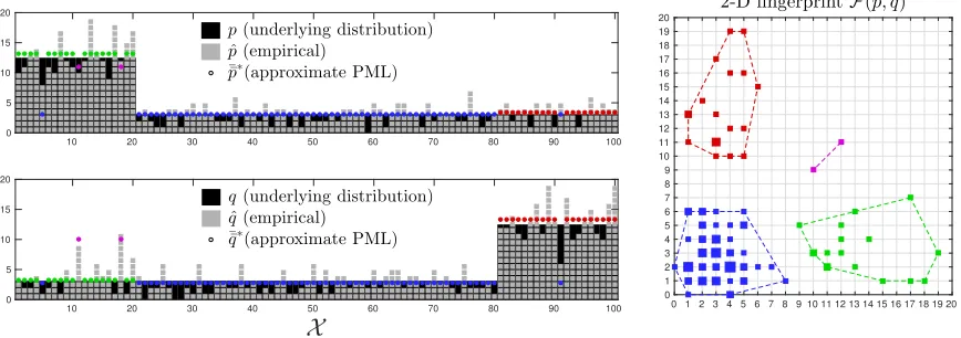
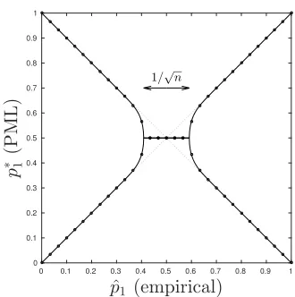
Figures 1 and 2 show the approximate PML distributions for the cases D = 1 and
D = 2, respectively. For D = 1, the approximate PML distribution is as defined in (23). ForD≥2, we approximately maximize our lower bound ¯V to the log matrix permanent as described in Appendix H. Figure 14 in Appendix H shows the case D= 3.
X
10 20 30 40
0 5 10 15 20
p(underlying distribution)
ˆ
p(sorted empirical)
¯
p∗(approximate PML)
X
5 10 15 20 25 30 35 40
X
5
10
15
20
25
30
35
40
Figure 1: (left) An empirical histogram ˆp sorted in non-increasing order (gray squares) drawn from underlying distribution p (black area) and the approximate PML (APML) distribution ¯p∗ (23) (red line), scaled by the sample size n = 200. The alphabet is X =
{1, . . . ,40}, assumed unknown in computing ¯p∗. (right) Computation of the log permanent
lower bound ¯V(¯p∗) (31) involves summing over all permutations that mix symbols only within the level sets of ¯p∗, corresponding to all permutation matrices with nonzero entries within the black blocks.
4.2. Intuitions from solving the PML exactly
For small alphabets, we can numerically and sometimes analytically optimize the permanent in (16) and (20). We observe that the PML distribution tends to assign equal mass to symbols whose empirical counts are close, differing on the order of √n, where n is the sample size. This observation motivates our approximate PML scheme in Section 4.3.
4.2.1. Exact solution for size 2 alphabet
Suppose the alphabet size is |X | = 2. Given sample size n and empirical distribution ˆ
10 20 30 40 50 60 70 80 90 100 0
5 10 15 20
p(underlying distribution)
ˆ
p(empirical)
¯¯
p∗(approximate PML)
X
10 20 30 40 50 60 70 80 90 100
0 5 10 15 20
q(underlying distribution)
ˆ
q(empirical)
¯¯
q∗(approximate PML)
012 34 567 89 10 11 12 13 14 15 16 17 18 19 20 0
1 2 3 4 5 6 7 8 9 10 11 12 13 14 15 16 17 18 19 20
2-DfingerprintF(ˆp,qˆ)
Figure 2: (Left) empirical distributions ˆp and ˆq (gray squares) drawn from underlying distributions p and q (black area) with n = m = 400 samples. The approximate PML distributions (¯p¯∗,q¯¯∗) are computed by clumping entries of a 2-D fingerprint according to the greedy heuristic described in Appendix H. The approximate PML distributions are ordered in the same way as the empirical distributions (with a distinct color for each level set corresponding to the subplot on the right). All distributions are plotted scaled by the sample size. (Right) the 2-D fingerprintFi,j at coordinates (i, j). Marker areas are roughly proportional toFi,j. All points within the colored convex hulls correspond to a level set of the approximate PML distributions. We can see three large level sets corresponding to the three distinct values of (px, qx) for x∈ X.
Theorem 7 ((Orlitsky et al., 2004b)) For all n1 ≤pˆ1≤ 12,
ˆ
p∗=
1 2,
1 2
:|pˆ1−pˆ2| ≤ √1n
1 1+p,
p 1+p
:|pˆ1−pˆ2|> √1n
, (26)
where p is the unique root in (0,1)of the polynomial
ˆ
p1pn(1−2 ˆp1)+1−pˆ2pn(1−2 ˆp1)+ ˆp2p−pˆ1. (27)
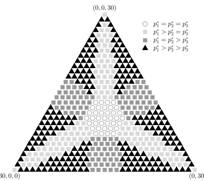
Theorem 7 states that |pˆ1−pˆ2| ≤ √1n ⇔ p∗ is uniform, which confirms our intuition that the relative ranking of two bins is “resolvable” if their empirical counts are more than about√napart, since the empirical counts are marginally binomially-distributed with standard deviation proportional to √n. Figure 3 summarizes these observations for the size-2 alphabet.
4.2.2. Size 3 alphabet
non-ˆ
p1 (empirical)
0 0.1 0.2 0.3 0.4 0.5 0.6 0.7 0.8 0.9 1
p
∗ 1
(P
M
L)
0 0.1 0.2 0.3 0.4 0.5 0.6 0.7 0.8 0.9 1
1/√n
Figure 3: “Phase diagram” for the PML distribution p∗ = (p∗1,1−p∗1) on binary alphabet
X = {1,2} and empirical distribution (ˆp1,1−pˆ1) on n = 30 samples (plotting the first component). Circles correspond to the possible histograms (ˆp1 ∈ {0/30,1/30, . . . ,30/30}). Solid black lines correspond to the solution for arbitrary ˆp1 ∈[0,1], obtained numerically. The PML distribution p∗ is uniform when |pˆ1 −pˆ2| ≤ 1/
√
n. Outside this middle region there are two PML branches, since any permutation of the PML distribution is another PML distribution. Diagonal dashed lines correspond to the lines (ˆp1,pˆ1) and (ˆp1,1−pˆ1).
increasing order and denote the result by p∗EM. Details of the EM algorithm can be found in Appendix D. We summarize our findings in Figure 4.
4.2.3. Exact solution for size 2 alphabet with D distributions
Suppose we have Ddistributions ((p(1d),1−p(1d)))D
d=1 on the same alphabetX ={1,2} and draw (nd)Dd=1samples from each, obtaining empirical distributions ((ˆp(1d),1−pˆ(1d)))Dd=1. Then the D-dimensional PML distribution (p∗(d))Dd=1 (defined for D = 2 in Section 3.2 and for generalD in Appendix H) is stated in Theorem 8.
Theorem 8 The D-tuple of PML distributions(p∗(d))Dd=1 on a binary alphabet satisfies:
D X d=1
4nd
ˆ
p(1d)− 1
2 2
>1 ⇒ (p∗(d))Dd=16=
1 2,
1 2
D
d=1
(28)
(30,0,0) (0,30,0) (0,0,30)
p∗
1=p∗2=p∗3
p∗
1> p∗2=p∗3 p∗
1=p∗2> p∗3 p∗
1> p∗2> p∗3
Figure 4: “Phase diagram” for the PML distribution approximationp∗EM for alphabet size
|X | = 3 bins and n = 30 samples (analogous to Figure 3), computed by an expectation-maximization (EM) algorithm as discussed in Section 4.2.2 and Appendix D. We plot a marker for each possible empirical distribution – a type – on the simplex. Each type has three coordinates, which we then project onto the 2-dimensional image shown (so, e.g., the uniform type npˆ= (10,10,10) is in the center). The shape of the marker at position npˆ corresponds to the level set decomposition of the distributionp∗EM, with components sorted in non-increasing order.
4.2.4. Empirical observations of the exact solutions
Figures 3, 4, and 5 suggest that the PML distribution tends to “cluster” together similar entries of the empirical histogram ˆp, rather than smooth them out. Ifn|pˆx−pˆx0|is smaller than approximately √npˆx, then the relative ranking of the true distribution’s x and x0 components is not well resolved statistically, and the permanent of Q (14) tends to be maximized with p∗x = p∗x0. On the other hand if n|pˆx−pˆx0| is larger than approximately
√
npˆx, then it tends to happen thatp∗x 6=p∗x0. The similar phenomenon of a phase transition between a uniform and nonuniform PML distribution (for a different approximation of the PML (Vontobel, 2012)) has been reported by (Fernandes and Kashyap, 2013; Chan et al., 2015).
These observations lead to the intuition that permutations σ ∈ SX that exchange
ˆ
p
1(empirical)
0 0.1 0.2 0.3 0.4 0.5 0.6 0.7 0.8 0.9 1ˆ
q
1(e
m
p
ir
ic
al
)
0 0.1 0.2 0.3 0.4 0.5 0.6 0.7 0.8 0.9 1
1/√n
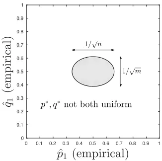
1/√m
p∗, q∗not both uniform
Figure 5: “Phase diagram” for the 2-D PML pair of distributions p∗, q∗ (20) on binary alphabet X ={1,2} and empirical distributions (ˆp1,1−pˆ1), (ˆq1,1−qˆ1) onn= 10, m= 20 samples. p∗, q∗ are not both uniform whenever the empirical distribution components ˆp1,qˆ1 both lie outside the shaded ellipse 4n pˆ1−122+ 4m qˆ1−122≤1.
4.3. Approximate PML: the case of a single distribution
In the sequel, denote byA(p) ={α} the partition ofX into the level sets ofp:
A(p),{{x∈ X :px=u}:u∈ {px :x∈ X }} (29)
In this Section we assume that the underlying distributionpis supported on finite setX
of known cardinality. The case of unknown or infinite support set size is treated in Section 4.6. If the support set size is known, then so is the number of “unseen” symbolsF0, so from (16) we conclude that the PML distribution p∗ is a maximizer of the function:
V(p),log(perm(Q)) (30)
We lower bound the log permanent V(p) by summing over a subset of the terms in the summation – a subgroup of the symmetric group SX. Denote the lower bound by ¯V(p):
¯
V(p),log
X σ∈SX,p
Y x∈X
pnxpˆσ(x) ≤log
X σ∈SX
Y x∈X
pnxpˆσ(x)
=V(p) (31)
where SX,p is a subgroup of SX consisting of all permutations that exchange only those
alphabet symbols x, x0 ∈ X that are within the same level set of p. Equivalently, SX,p is the stabilizer of distributionp under the action of relabeling its components:
SX,p,{σ∈ SX :σp=p} ∼=
×
α∈A(p)
Sα (32)
where (σp)x ,pσ(x),∼= denotes group isomorphism,×denotes the direct product of groups, and Sα is the symmetric group acting on level setα ⊂ X. Then|SX,p|=
Q
Our approximate profile maximum likelihood distribution ¯p∗maximizes the lower bound ¯
V(p). In other words, for the case of every distribution in collection P having the same support set size,
¯
p∗,argmax p∈P
¯
V(p) (33)
The case of unknown support set size is treated in Section 4.6.
Some intuition for the computational difficulty of the proposed approximation: the product structure (32) ofSX,p allows us to lower bound the log matrix permanent V(p) = log(perm(Q)) ≥ log(perm( ¯Q)) = ¯V(p), where ¯Q is the block-diagonal matrix ¯Qx,x0 =
Qx,x01(ˆpx= ˆpx0) whose permanent is the product of the permanents in each block. Sincep is constant within each block, the permanent of each block is easy to evaluate, so evaluation of the lower bound ¯V(p) is dramatically simpler than evaluation ofV(p), taking timeO(|X |). It moreover turns out to be possible to optimize ¯V(p) computationally efficiently to find the approximate PML distribution ¯p∗; this is done below.
The restriction to summing over SX,p rather thanSX seems large, but the hope is that
¯
p∗ clusters together only comparably frequent symbols (that is, ¯p∗x= ¯p∗x0 impliesn|pˆx−pˆx0| is less than about√npˆx), so we hope that ¯V(¯p∗)≈V(¯p∗) and that ¯p∗ is close top∗, the exact profile maximum likelihood (16). Figure 1 shows that the approximate PML distribution ¯p∗
clustering together similar enough bins of ˆp. We thus expect our approximate PML scheme to perform best when data is drawn from a distribution with a few well-separated level sets (like a uniform distribution or mixture of uniforms) and less well for more smoothly-varying distributions (like a Zipf distribution); this intuition is borne by the numerical experiments of Section 5.
We can rewrite our log permanent lower bound ¯V(p) (31) as (see proof in Appendix F):
¯
V(p) = log
X σ∈SX,p
Y x∈X
pnpˆσ(x)
x
(34)
=−n D(ˆp||p) +H(ˆp)+ X α∈A(p)
log(|α|!) (35)
where A(p) (29) is the partition of X into level sets of p, D(ˆp||p) is the Kullback-Leibler divergence and H(ˆp) is the entropy of the empirical distribution.
Expression (35) yields some intuition about the approximate PML distribution ¯p∗ – a maximizer of ¯V(p). A distribution p that “clumps” many symbols together (that is, has a few large level sets α) boosts the second term (the summation over α ∈ A(p)) in (35), but is very different from ˆp, thus lowering the first term. On the other hand, by setting
p= ˆp, we maximize the first term, but reduce the second term. As the sample size n→ ∞, the contribution of the second term in (35) vanishes relative to the first term, and we have ¯
p∗ →pˆ, the ML distribution, in this limit.
4.4. Properties of the approximate PML distribution
Letα⊂ X and denote by ˆpα the average value of the empirical distribution ˆp overα:
ˆ
pα ,
1
|α|
X x∈α ˆ
px (36)
We can show that the PML distribution approximation ¯p∗ (33) satisfies for allx∈ X
¯
p∗x= ˆpα(x,p¯∗) (37)
where α(x,p¯∗) = {x0 :∈ X : ¯px∗0 = ¯p∗x} is the level set of ¯p∗ containing x. That is, ¯p∗x (37) is equal to the average value of the empirical histogram ˆp over the symbols clumped with x into the same level set of ¯p∗. This follows from the fact that D(ˆpkp) is a Bregman divergence (Jiao et al., 2017, Lemma 4).
The averaging property (37) determines our approximate PML distribution ¯p∗ in terms of its partition of X into level sets. Therefore, instead of maximizing ¯V(p), we maximize
¯
V(A), defined:
¯
V(A), X
α∈A
¯
V(α) (38)
where forα⊂ X
¯
V(α),log (|α|!) +n|α|pˆαlog(ˆpα) (39)
We can check that ¯V(A) = ¯V(ˆpA), where ˆpA is the distribution obtained by averaging the
empirical distribution ˆp within each partition element α ∈ A. Let ¯A∗ denote the optimal partition:
¯
A∗ , argmax
A: partition ofX
¯
V(A) (40)
Now optimizing the lower bound to the permanent ¯V(p) (31) is equivalent to optimizing ¯
V(A) (38) over partitions ofX, since ¯V(¯p∗) = ¯V( ¯A∗) and ¯p∗ = ˆpA¯∗.
We make two observations for the solution of the approximate PML problem (40) that allow us to restrict the set of partitions over which we optimize. LetAbe a partition ofX. We sayA has theiso-clumping orconvexity properties defined below:
1. Iso-clumping property. Symbols with the same empirical probabilities are clumped together: For allx, x0 ∈ X:
ˆ
px = ˆpx0 ⇒α(x) =α(x0) (41)
Whereα(x)∈ Ais the partition element containing x.
2. Convexity property. For allx, x0, x00∈ X:
ˆ
px<pˆx0 <pˆx00 and α(x) =α(x00)
⇒α(x) =α(x0) =α(x00) (42)
Theorem 9 Let A¯∗ (40) be the partition of X into level sets of the approximate PML distribution p¯∗ (33) and let pˆbe the empirical distribution. Then A¯∗ has the iso-clumping and convexity properties (41) and (42).
4.5. A dynamic programming computation of the approximate PML distribution
Theorem 9 lets us efficiently maximize ¯V(A) (38) by restricting to only those partitions of
X that have the iso-clumping and convexity properties. Once we find ¯A∗(40), the averaging property (37) lets us compute the approximate PML distribution ¯p∗.
Let F+ ,(Fi)i≥1. Let
0 =m0 < m1 < m2< . . . < mF+ ≤n (43)
where
Supp(F+) ={m≥1 :Fm >0}={mi}Fi=1+ (44) Then any distribution whose level set partition satisfies the iso-clumping (41) and con-vexity (42) properties has all level sets of the form Xi:j with 0≤i≤j≤F+:
Xi:j ,{x∈ X :mi≤npˆx≤mj}. (45)
Thus we optimize ¯V(A) (38) over partitions ofX into level sets of the form (45). Note that if F0 >0, then the set X0:0 ={x∈ X : ˆpx = 0} of unseen symbols can not appear in the optimal partition ¯A∗ because if it does, then its probability mass under pA¯∗ is 0, violating our assumption thatp has support X. IfF0= 0, then X0:0=∅.
This optimization can be done by a dynamic programming algorithm. For integersi≤j, let [i, j],{k∈N:i≤k≤j}. Let ¯Vi denote for 0≤i≤F+:
¯
Vi , max
j∈[i∨1,F+]
( ¯V(Xi:j) + ¯Vj+1) (46) (a)
= max
A: partition ofXi:F+
¯
V(A) (47)
with boundary condition ¯VF++1,0, wherei∨j denotes the greater ofi andj, and where
¯
V(Xi:j) is as in (39). (a) follows by induction onidownwards fromF+. We letj∈[i∨1, F+] in (46) (rather than j ∈[i, F+]) in order to optimize over only those partitions of X that do not contain the setX0:0 of unseen symbols; this restriction forces the approximate PML distribution to have support set size|X |, as we assumed in the beginning of Section 4.3.
Then the PML distribution approximation ¯p∗ = argmaxpV¯(p) satisfies (setting i = 0 and using X0:F+ =X in (47)):
¯
V(¯p∗) = max
A: partition ofX
¯
V(A) = ¯V0 (48)
We can compute the term ¯V(Xi:j) in (46), corresponding to clustering all symbols of
Xi:j into a level set ofp, using (39): ¯
V(Xi:j) = log (|Xi:j|!) +n|Xi:j|pˆXi:jlog ˆpXi:j
(49)
= log j X k=i
Fmk! !
+ j X k=i
mkFmk
! log
Pj
k=imkFmk
nPj
k=iFmk
!
(50)
where we used |Xi:j|=Pjk=iFmk and ˆpXi:j =
1 n|Xi:j|
Pj
Relations (46) and (50) allow us to compute the level set decomposition ¯p∗ by filling out a (F++ 1)×F+ array ( ¯V(Xi:j))i∈[0,F+],j∈[1,F+] and keeping track of the maximizing index
each time we compute ¯Vi. Once we have the optimal level set decomposition ¯A∗ = {Xi:j} of ¯p∗, we set for allx∈ Xi:j, for all i,j
¯
p∗x= ˆpXi:j (51)
For example, in Figure 1, we have (mi)F+=12
i=0 = (0,1,2,3,4,5,7,9,12,13,15,16,20) and the approximate PML distribution ¯p∗ (red line) has level sets{X0:6,X7:12}.
The running time of this dynamic programming algorithm is O(|Supp(F)|2), where
|Supp(F)| ≤F++ 1. In terms of the sample size n, any empirical distribution ˆp satisfies
|Supp(F(ˆp))| ≤ 1 2 1 +
√
8n+ 1
, with equality achieved by the empirical distribution ˆpi= 2i
|X |(|X |+1) fori∈[0,|X |] with |X |=|Supp(F)|andn= 1
2|X |(|X |+ 1). Thus the worst-case run time for the dynamic programming algorithm is O(√n2) =O(n). We “usually” have
|Supp(F)|much smaller than √n, so this is a pessimistic estimate for a typical case. The run time of our approximate PML scheme is usually dominated by computation of ˆp. An implementation optimization is to pre-compute the sums Pj
k=iFmk and
Pj
k=imkFmk for
all i≤j in computing ¯V(Xi:j).
4.6. Unknown or infinite support set size
If the support set sizeK=|X |is unknown, then we can attempt to infer it. Our estimator ¯
K∗ for the support set size is the same as (17), but replaces the permanent with our lower bound (31), eV¯(p)≤perm(Q):
¯
K∗ ,argmax K
1
(K−Kˆ)!pmax∈PK eV¯(p)
!
(52)
whenever the max over K exists, where PK , {p ∈ P : |Supp(p)| =K}, where ˆK = |X |ˆ is the support set size of the empirical distribution ˆp. Then the PML distribution is ¯p∗
with support set ¯K∗. The max over p is obtained via our approximate PML algorithm in Section 4.5. The maximizer ¯K∗ usually exists because a largerKboosts the value of the log permanent lower bound ¯V(p) (since there are more permutations to sum over), but reduces the first factor in (52). It may happen that ¯K∗ does not exist, in which case we say our approximate PML distribution has a continuous part in the terminology of (Orlitsky et al., 2004b). In general the function in the argmax in (52) is multimodal in K.
It turns out we can efficiently compute ¯K∗ if it exists and compute the corresponding approximate PML distribution; if ¯K∗ does not exist, then we can efficiently detect this case and compute the corresponding approximate PML distribution, which in this case has a continuous part.
We state and derive our observations in Appendix J. The idea is to optimize over all possible ways to clump the unseen symbolsX0:0 with the other symbols. Since the optimal clumping satisfies the iso-clumping and convexity properties, we show that there are only
4.7. Approximate PML: the case of multiple distributions (see Appendix H)
We generalize the PML distribution and approximate PML distribution to the case of (nd)Dd=1 samples drawn from distributions (p(d))Dd=1 on the same alphabet (see Section 3.2 for the case D= 2, used in estimating functionals of pairs of distributions). This requires some more notation that we delegate to Appendix H.
For D≥2, we are unable to give an efficient algorithm to compute the D-dimensional approximate PML. The difficulty is due to the lack of a natural ordering onND forD≥2,
so the dynamic programming approach we use forD= 1 does not work forD≥2. We settle for approximately computing our the approximate PML distribution via a greedy heuristic: we iteratively enlarge level sets of a candidate solution by merging pairs of distinct level sets until the objective function ¯V (suitably generalized toDdistributions) stops increasing. See Appendix H for details.
4.8. Comparison to the (exact) PML distribution for size 2 alphabet
Recall the discussion of Section 4.2.1 on the PML distribution for alphabet size|X |= 2. A computation establishes the condition for uniformity of the APML distribution:
¯
p∗=
( 1 2,
1 2
:H(ˆp)≥log(2) 1− 1 n
(ˆp1,1−pˆ1) : otherwise
(53)
whereH(ˆp) is the entropy of the empirical distribution and nis the sample size.
Let’s consider the large n limit. Let ˆpunif1 be the critical value at which the APML distribution switches between uniform and nonuniform (the least value of ˆp1 satisfying the uniformity condition in (53)). Then a computation shows that
ˆ
punif1 = 1
2 1− r
log(4)
n +O
1
n
!
(54)
Comparing this to condition (26) for the (exact) PML, we see that in the APML case, ˆpunif1
carries an extra factor ofplog(4)≈1.18 in the 1/√nterm relative to the uniform/nonuni-form critical value of ˆp1 for the PML.
Figure 6 compares the APML and PML distributions for a size-2 alphabet. Both the APML and PML are uniform when|pˆ1−pˆ2|is small enough, though at different points, as remarked above. Whenever the APML solution is not uniform, it exactly matches (up to relabeling of components) the empirical distribution, unlike the PML.
5. Estimating symmetric functionals of a single discrete distribution
In the standard PML setting discussed in Section 3.1, we argued the sufficiency of the fingerprint F (11) in estimating the sorted probability vector of a discrete distribution, which implies the sufficiency of the fingerprint for estimating any functionalF of the sorted probability vector of the form
F(p) =G X
x∈X
f(px)
ˆ
p1 (empirical)
0 0.1 0.2 0.3 0.4 0.5 0.6 0.7 0.8 0.9 1 0
0.1 0.2 0.3 0.4 0.5 0.6 0.7 0.8 0.9 1
n= 10
ˆ
p1 (empirical)
0 0.1 0.2 0.3 0.4 0.5 0.6 0.7 0.8 0.9 1 0
0.1 0.2 0.3 0.4 0.5 0.6 0.7 0.8 0.9 1
n= 30
p∗1 (PML)
¯
p∗1 (APML)
ˆ
p1 (empirical)
0 0.1 0.2 0.3 0.4 0.5 0.6 0.7 0.8 0.9 1 0
0.1 0.2 0.3 0.4 0.5 0.6 0.7 0.8 0.9 1
n= 100
Figure 6: “Phase diagram” for the exact PML (hollow circles) and APML distributions (red circles) on binary alphabet with sample sizen indicated above each subplot (compare to Figure 3). Solid black lines correspond to the solution for arbitrary ˆp1 ∈[0,1], obtained numerically. The PML distributionp∗ is uniform when|pˆ1−pˆ2| ≤1/
√
n, while the APML distribution is uniform when|pˆ1−pˆ2| ≤
p
log(4)/√n+O(1/n). Outside this middle region there are two PML (APML) branches, since any permutation of the PML (APML) distri-bution is another PML (APML) distridistri-bution. The APML distridistri-bution exactly matches the empirical distribution outside the uniform region. Diagonal dashed lines correspond to the lines (ˆp1,pˆ1) and (ˆp1,1−pˆ1).
where we constrainf(0) = 0 to accommodate the unknown alphabet setting. Note that the fingerprint is also partially sufficient for functionals of typeP
x,y∈Xf(px, py), etc.
In order to apply Theorem 3, one also needs to show the cardinality of the fingerprint
F is small. The fingerprint F = (Fi)i≥0 satisfies X
i≥0
iFi =n, (56)
and each fingerprint corresponds to an unordered integer partition of the integer n. We now recall the Hardy-Ramanujan result on integer partitions.
Theorem 10 (Hardy and Ramanujan, 1918)(B´ar´any and Vershik, 1992, Theorem 2) The cardinality of the set of fingerprints (11) on n samples is given by
eπ
q 2n
3 (1−o(1)) ≤ |{(Fi)i
≥1}| ≤eπ
q 2n
3 . (57)
The key observation is that the cardinality of the fingerprint is sub-exponential. Then, combining with Theorem 3 and the fact that there exist estimators for various symmetric functionals with near exponential measure concentration, (Acharya et al., 2017) showed that plugging in the PML achieves the optimal sample complexity in estimating the Shannon entropy, the support size, the support coverage, and theL1 distance to uniformity.
that the PML distributionp∗ is defined as in (16) for empirical distribution ˆponnsamples with fingerprint F(ˆp):
p∗= argmax p∈P Pp
(F) = argmax p∈P
perm
pnpˆx0
x
x,x0∈X
(K−Kˆ)! . (58)
where the optimization is over distributions of possibly different support set size,X denotes the support set of distribution p, K = |X |, and ˆK denotes the support set size of the empirical distribution ˆp. p∗ is difficult to compute exactly, so we compute the APML distribution ¯p∗ (33), (52):
¯
p∗ = argmax p∈P
eV¯(p)
(K−Kˆ)! (59)
which maximizes a lower bound to the probability Pp(F) since ¯V(p) (31) lower bounds the log permanent in (58). Then our estimator for function F of the form (55) is the plugin
F(¯p∗).
Our approximate PML estimator performs comparably well to the competition (Valiant and Valiant, 2011a) (Valiant and Valiant, 2013) (Jiao et al., 2015), (Wu and Yang, 2016), (Wu and Yang, 2015) across different functions F and distributions, and performs signifi-cantly better when the true distribution is uniform. This good performance for the uniform case makes some intuitive sense: the approximate PML distribution ¯p∗ maximizes a lower bound (22) to a matrix permanent obtained by summing over only those permutations that mix symbols within level sets of ¯p∗. If there is only one level set – that is, if ¯p∗ is uniform – then we have exactly optimized the matrix permanent (or at least found a local maximum), rather than a lower bound to the permanent.
5.1. Sorted L1 loss
Given n samples from a distribution p, the usual L1 loss in measuring the accuracy of estimatingp is given by
X x∈X
|px−qx|. (60)
The sortedL1loss measures theshapedifference between the reconstruction distribution
q and the true distributionp. In other words, we first sort the distributions p, q into non-increasing probability vectors (p(1), p(2), . . . , p(K)),(q(1), q(2), . . . , q(K)), and then measure the loss by
X 1≤i≤K
|p(i)−q(i)|. (61)
The sorted L1 loss measures the error in reconstructing the sorted probability vector, for which the fingerprints are partially sufficient as shown by Theorem 6. The sorted L1 loss can also be viewed as a Wasserstein distance (Vallender, 1974), i.e.,
X 1≤i≤K
|p(i)−q(i)|=K sup f∈Lip1
Z
f(x) X
x 1
Kδpx−
X x
1
Kδqx
!
where the supremum is over all Lipschitz functions with Lipschitz constant one.
We estimate the sorted L1 loss using the plug-in q = ¯p∗, the APML distribution (59), computed over collection of distributions P = ∆, where
∆,{p:|Supp(p)|<∞} (63)
denotes the set of all discrete distributions with finite support set size, and collection of distributions P = ∆K, where
∆K,{p:|Supp(p)|=K} (64)
denotes the set of all discrete distributions with support set size K.
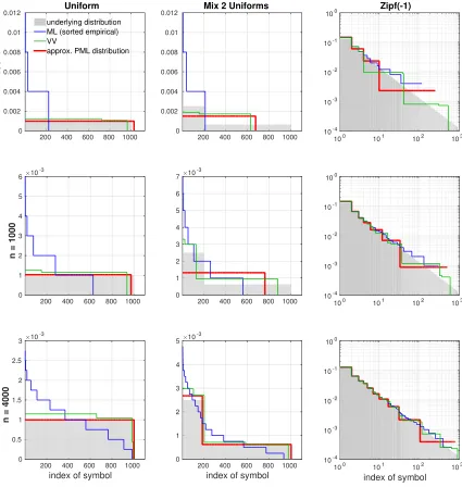
Figure 7 shows the sorted probability vector inferred by our approximate PML distri-bution in ∆ (63) – that is, the case of unknown support set size – along with the sorted ML (empirical) distribution and the distribution of (Valiant and Valiant, 2013). We see that both the approximate PML distribution and the distribution of (Valiant and Valiant, 2013) perform much better than the sorted ML distribution, and that the PML distribution “prefers” to have fewer and larger level sets than the distribution of (Valiant and Valiant, 2013).
200 400 600 800 1000
n = 250
0 0.002 0.004 0.006 0.008 0.01
0.012 Uniform
underlying distribution ML (sorted empirical) VV
approx. PML distribution
200 400 600 800 1000
n = 1000
×10-3
0 1 2 3 4 5 6
index of symbol
200 400 600 800 1000
n = 4000
×10-3
0 0.5 1 1.5 2 2.5 3
200 400 600 800 1000 0
0.002 0.004 0.006 0.008 0.01
0.012 Mix 2 Uniforms
200 400 600 800 1000
×10-3
0 1 2 3 4 5 6 7
index of symbol
200 400 600 800 1000
×10-3
0 1 2 3 4 5
100 101 102 103 10-4
10-3 10-2 10-1
100 Zipf(-1)
100 101 102 103 10-4
10-3 10-2 10-1 100
index of symbol
100 101 102 103 10-4
10-3 10-2 10-1 100
sample size
102 104 106 108 10-6
10-4 10-2 100
102 Uniform
sample size
102 104 106 108 10-4
10-3 10-2 10-1 100
101 Mix 2 Uniforms
sample size
102 104 106 108 10-3
10-2 10-1 100
101 Zipf(-1)
sample size
102 104 106 108 10-3
10-2 10-1 100
101 Zipf(-0.6) MLE
VV
this work
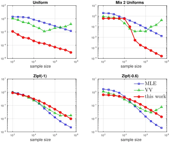
Figure 8: SortedL1loss in estimating an unknown distributionpwith known support set size
K =|X |. In all casesK = 104. “Uniform” is uniform onX, “Mix 2 Uniforms” is a mixture of two uniform distributions, with half the probability mass on the firstK/5 symbols, and the other half on the remaining symbols, and Zipf(α) ∼ 1/iα with i ∈ {1, . . . , K}. MLE denotes the ML plugin (“naive”) approach of using the sorted empirical distribution in (61). VV is (Valiant and Valiant, 2013). Each data point represents 100 random trials, with 2 standard error bars smaller than the plot marker for most points.
5.2. Entropy and R´enyi entropy estimation
For entropy H(p) =−P
x∈Xpxlog(px) and R´enyi entropy Hα(p) = 1−1αlog Px∈Xpαx
of distributionp, the corresponding approximate PML estimator is defined as the plugin esti-matorH(¯p∗), Hα(¯p∗), where ¯p∗ is as in (59), optimized over the collection of distributions
P = ∆ (63) for both the entropy and R´enyi entropy. Additionally, to enable direct com-parison with the entropy estimator of (Wu and Yang, 2016), which requires a support set size as input, we also find the approximate PML distribution optimized overP = ∆K (64).
102 104 106 108 Uniform 10-6 10-4 10-2 100 entropy MLE VV JVHW this work WY (known|X |) this work (known|X |)
102 104 106 108
Mix 2 Uniforms
10-4 10-2 100 102 104 106 108 Zipf(-1) 10-3 10-2 10-1 100
102 104 106 108
Zipf(-0.6)
10-4
10-2
100
sample size
102 104 106 108
Geometric
10-4
10-2
100
102 104 106 108
10-6
10-4
10-2
100
R´enyi entropy (α= 2)
102 104 106 108
10-3 10-2 10-1 100 101 102 104 106 108 10-3 10-2 10-1 100
102 104 106 108
10-3
10-2
10-1
100
sample size
102 104 106 108
10-3
10-2
10-1
100
101
102 104 106 108
10-6
10-4
10-2
100
R´enyi entropy (α= 1
.5)
102 104 106 108
10-3 10-2 10-1 100 101 102 104 106 108 10-3 10-2 10-1 100
102 104 106 108
10-3 10-2 10-1 100 101 sample size
102 104 106 108
10-3
10-2
10-1
100
101
102 104 106 108
10-6
10-4
10-2
100
R´enyi entropy (α= 0
.8)
102 104 106 108
10-4 10-3 10-2 10-1 100 101 102 104 106 108 10-3 10-2 10-1 100 101
102 104 106 108
10-3 10-2 10-1 100 101 sample size
102 104 106 108
10-2
10-1
100
101
Figure 9: Root mean squared error of several estimators of entropy (first column) and R´enyi entropy (last three columns forα∈ {2,1.5,0.8}). In all cases except “Geometric” we set the alphabet size |X |= 104. “Uniform” is uniform onX, Zipf(α) ∼1/iα withi∈ {1, . . . , K}, “Geometric” is the geometric distribution with infinite support and meanK. MLE denotes the ML plugin (“naive”) approach of computingH(ˆp). VV is (Valiant and Valiant, 2013). JVHW is (Jiao et al., 2015). WY is (Wu and Yang, 2016) – this estimator requires the support set size|X | as an input. Our estimator optionally accepts the support set size|X |
5.3. L1 distance to uniformity
For estimating the L1 distance to uniformity, which is Px∈X|px−K1|, the corresponding PML estimator is (Acharya et al., 2017) the plugin of p∗ (58) optimized over the collection of distributions P = ∆K (64) (the case of known support set size). The APML estimator is the plugin of ¯p∗ (59) optimized overP = ∆K.
Figure 10 shows the performance of our approximate PML scheme for estimating the
L1 distance to a uniform distribution with known support set size. Our approach looks competitive, and is by far the best if the true distribution is uniform.
sample size
102 104 106 108
10-5
10-4
10-3
10-2
10-1
100
101 Uniform
sample size
102 104 106 108
10-4
10-3
10-2
10-1
100
101 Mix 2 Uniforms
sample size
102 104 106 108
10-4
10-3
10-2
10-1
100 Zipf(-1)
sample size
102 104 106 108
10-4
10-3
10-2
10-1
100
101 Zipf(-0.6) MLE
VV
this work
Figure 10: Root mean squared error for estimation ofL1 distance to uniformity with known support set size K = |X |. In all cases K = 104. “Uniform” is uniform on X, “Mix 2 Uniforms” is a mixture of two uniform distributions, with half the probability mass on the firstK/5 symbols, and the other half on the remaining symbols, and Zipf(α)∼1/iαwithi∈
{1, . . . , K}. MLE denotes the ML plugin (“naive”) approach of computingP
5.4. Support set size estimation
For support size estimation, the corresponding PML estimator is (Acharya et al., 2017) the plugin of p∗ (58) optimized over the collection of distributions P = ∆≥1
K, where
∆≥1
K ,
{p:px≥ 1
K ∀x∈ X } (65)
denotes the set of all discrete distributions whose minimum nonzero probability for each symbol is at least K1. The approximate PML estimator is the plugin of ¯p∗ (59) optimized overP = ∆≥1
K.
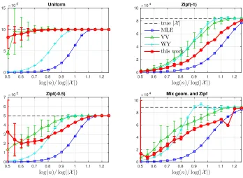
Figure 11 shows the performance of our approximate PML scheme for estimating the support set size. Here we plot the mean and standard error of the support set size inferred by the different estimation schemes rather than a root mean squared error. Overall, our approach is comparable to the others, performing worst on the Zipf distributions, and best on the uniform distribution.
log(n)/log(|X |)
0.5 0.6 0.7 0.8 0.9 1 1.1 1.2
×105
0 5 10
15 Uniform
log(n)/log(|X |)
0.5 0.6 0.7 0.8 0.9 1 1.1 1.2
×104
0 2 4 6 8
10 Zipf(-1)
true|X |
MLE VV WY this work
log(n)/log(|X |)
0.5 0.6 0.7 0.8 0.9 1 1.1 1.2
×105
0 1 2 3 4 5 6
7 Zipf(-0.5)
log(n)/log(|X |)
0.5 0.6 0.7 0.8 0.9 1 1.1 1.2
×104
0 2 4 6 8 10
Mix geom. and Zipf
Figure 11: Support set size estimation for the same cases as in (Wu and Yang, 2015), plotting the mean and 2 standard deviations of the distribution of inferred support set sizes in 100 trials vs. sample size n. In all cases the support set set size K = |X | is chosen such that mini∈{1,...,K}pi ≈10−6. “Uniform” is uniform on{1, . . . , K}, Zipf(α)∼1/iαwith
i∈ {1, . . . , K}, and “Mix geom. and Zipf” is a mixture ofpi∼1/ifori∈ {1, . . . , K/2}and
6. Estimating the divergence function between two distributions
In the 2-D PML setting discussed in Section 3.2, we argued the sufficiency of the finger-print (18) in estimating functions of two discrete distributions of the form
F(p, q) =X
x∈X
f(px, qx). (66)
In order to apply Theorem 3, one needs to show the cardinality of the sufficient statistic is not too big. Below we present an argument that applies to theD-dimensional PML. Suppose we have D discrete distributions on the same alphabet X, denoted as p(1), p(2), . . . , p(D). Suppose we obtain ndsamples from each distribution p(d) with empirical distribution ˆp(d). Let the joint fingerprint be defined for every (i1, i2, . . . , iD)≥0,
Fi1,i2,...,iD =|{x∈ X : (ndpˆ
(d)
x )Dd=1= (id)Dd=1}|. (67) We now argue that the joint fingerprint (Fi1,i2,...,iD)(i1,i2,...,iD)≥0 corresponds to the
par-tition of multipartite numbers. Indeed, the joint fingerprint satisfies the following equation:
X (i1,i2,...,iD)≥0
Fi1,i2,...,iD
i1
i2 .. .
iD
=
n1
n2
.. .
nD
. (68)
Theorem 11 quantifies the size of the sufficient statistic.
Theorem 11 (Auluck, 1953; B´ar´any and Vershik, 1992; Acharya et al., 2011) Suppose
D= 2. If n1 =n2 =n, then the cardinality of the set of 2-D fingerprints on n samples is
given by
|{(Fij)(i,j)=(06 ,0)}|=e3(ζ(3))
1/3n2/3(1+o(1))
. (69)
For general D >2, if nd≥2D+1,1≤d≤D, we have
|{(Fi1,i2,...,iD)(i1,i2,...,iD)6=0}| ≤exp 2
1 + 1
D
D X d=1
n D
D+1
d !
. (70)
where 0= (0, . . . ,0). Moreover, ifnd=n for alld∈ {1, . . . , D}, we have
|{(Fi1,i2,...,iD)(i1,i2,...,iD)6=0}|= exp
(D+ 1)(ζ(D+ 1))1/(D+1)nDD+1(1−o(1))
. (71)
Here ζ(D+ 1) =P∞
k=1k−(D+1) is the Riemann zeta function.
Han et al., 2016a,b; Bu et al., 2016; Valiant and Valiant, 2011a; Jiao et al., 2018)), we know that plugging in the 2-D PML achieves the optimal sample complexity in estimating the Kullback-Leibler divergence, L1 distance, the squared Hellinger distance, and the χ2 divergence. The proof of these results is to be reported elsewhere.
In this section, we extensively test the performance of divergence estimation via plugging in our approximate 2-D PML. We mainly compete with the released code of KL divergence estimator in (Han et al., 2016a,b). The concrete divergence functional estimation algorithm is as follows. Suppose we observensamples from distributionpwith empirical distribution ˆ
p and m samples from distribution q with empirical distribution ˆq. Let the 2-D PML estimator be as (20):
(p∗, q∗) = argmax (p,q)∈P
Pp,q(F), (72)
where F is the 2-D fingerprint (18) and P is a collection of pairs of distributions on the same alphabet X. The APML distributions maximize a lower bound toPp,q(F):
(¯p∗,q¯∗) = argmax (p,q)∈P
eV¯(p,q)
(K−Kˆ)! (73)
where ¯V is defined for the D-dimensional case in Appendix H, X = Supp(p)∪Supp(q),
K =|X |, and ˆK=|Supp(ˆp)∪Supp(q)|.
As discussed in Section 4.7, there is no natural ordering on the bins of the 2-D finger-print, so we do not give a dynamic programming algorithm like the one in section 4.5 to find the APML distributions. Instead we use a greedy heuristic presented in Appendix H to approximately maximize ¯V(p, q) and approximate the already-approximate PML distri-butions:
(¯p¯∗,q¯¯∗)≈(¯p∗,q¯∗) (74)
Then our estimator for functional F of the form (66) isF(¯p¯∗,q¯¯∗).
Our approximate PML estimator performs overall best relative to the competition, which for the KL divergence consists of only (Han et al., 2016a,b) and the MLE plugin estimator, and for the L1 distance consists of only the MLE plugin estimator. (Valiant and Valiant, 2013), (Valiant, 2008) generalize their approach to the 2-D fingerprint setting, but do not release code to repeat their experiments.
6.1. KL divergence estimation
For the KL divergence D(p||q) = P
x∈Xpxlog
px
qx
, the corresponding approximate PML estimator is the plugin D(¯p¯∗||q¯¯∗), where ¯p¯∗,q¯¯∗ are as in (74), optimized over collection of distributions P = ∆ρ, where
∆ρ={(p, q) : sup x
(px/qx)≤ρ} (75)
denotes the set of all pairs of discrete distributions with finite support and maximum ratio
ρ.