Using Side Information to Reliably Learn Low-Rank Matrices from Missing and Corrupted Observations

(1)

Using Side Information to Reliably Learn Low-Rank

Matrices from Missing and Corrupted Observations

Kai-Yang Chiang [email protected]

Inderjit S. Dhillon [email protected]

Department of Computer Science University of Texas at Austin Austin, TX 78701, USA

Cho-Jui Hsieh [email protected]

Department of Statistics and Computer Science University of California at Davis

Davis, CA 95616, USA

Editor:Sanjiv Kumar

Abstract

Learning a low-rank matrix from missing and corrupted observations is a fundamental problem in many machine learning applications. However, the role ofside information in low-rank matrix learning has received little attention, and most current approaches are either ad-hoc or only applicable in certain restrictive cases. In this paper, we propose a general model that exploits side information to better learn low-rank matrices from missing and corrupted observations, and show that the proposed model can be further applied to several popular scenarios such as matrix completion and robust PCA. Furthermore, we study the effect of side information on sample complexity and show that by using our model, the efficiency for learning can be improved given sufficiently informative side information. This result thus provides theoretical insight into the usefulness of side information in our model. Finally, we conduct comprehensive experiments in three real-world applications— relationship prediction, semi-supervised clustering and noisy image classification, showing that our proposed model is able to properly exploit side information for more effective learning both in theory and practice.

Keywords: Side information, low-rank matrix learning, learning from missing and cor-rupted observations, matrix completion, robust PCA

1. Introduction

Learning a low-rank matrix from noisy, high-dimensional complex data is an important research challenge in modern machine learning. In particular, in the recent big data era, assuming that the observations come from a model with implicit low-rank structure is one of the most prevailing approaches to avoid the curse of dimensionality. While various low-rank matrix learning problems arise from different contexts and domains, the primary challenge is rather similar: namely to reliably learn a low-rank matrix L0 based only on missing and corrupted observations from L0. This generic framework includes many well-known

machine learning problems such as matrix completion (Cand`es and Tao, 2009), robust PCA (Wright et al., 2009) and matrix sensing (Zhong et al., 2015), and is shown to be

c

(2)

useful in many important real-world applications including recommender systems (Koren et al., 2009), social network analysis (Hsieh et al., 2012) and image processing (Wright et al., 2009).

Among research related to low-rank matrix learning, one promising direction is to fur-ther exploitside information, orfeatures, to help the learning process. 1 The notion of side information appears naturally in many applications. For example, in the famous Netflix problem where the goal is movie recommendation based on users’ ratings, a popular ap-proach is to assume that the given user-movie rating pairs are sampled from a low-rank matrix (Koren et al., 2009). However, besides rating history, profiles of users and/or genres of movies may also be provided, and one can possibly leverage such side information for better recommendation. Since such additional features are available in many applications, designing a model to better incorporate features into low-rank matrix learning problems becomes an important issue with both theoretical and practical interests.

Motivated by the above realization, we study the effect of side information on learning low-rank matrices from missing and corrupted observations in this paper. Our general problem setting can be formally described as follows. Let L0 ∈ Rn1×n2 be the low-rank

modeling matrix, yet due to various reasons we can only observe a matrix R ∈ Rn1×n2

which contains missing and/or corrupted observations of L0. In addition, suppose we are also given additional feature matricesX ∈_Rn1×d1 _and/or _Y _∈

Rn2×d2 as side information,

where each row xi ∈ Rd1 (or yi ∈ Rd2) denotes a feature representation of the i-th row

(or column) entity of X (or Y). Then, instead of just using R to recover L0, our hope is to leverage side information X and Y to learn L0 more effectively. Below, we further list

some important applications where the side information naturally comes in as the form of

X and/or Y in this framework:

• Collaborative filtering. Collaborative filtering is one of the most popular machine

learning applications in industry where we aim to predict the preferences of users to any products based on limited rating history (e.g. the Netflix problem we mentioned previously). A traditional approach is to complete the partial user-product rating matrixR via matrix completion. However, one could also collect per-user features xi

and per-product features yj as possible information to leverage, and the assembled

feature representation for users and products becomesX and Y in this framework.

• Link prediction. The link prediction problem in online social network analysis is to

predict and recommend the implicit friendships of users given the current network snapshot. One approach is to think of the network snapshot as a user-to-user rela-tionship matrixR, and thus any missing relationships in the snapshot can be inferred by conducting matrix completion onR(Liben-Nowell and Kleinberg, 2007). Similarly, if user-specific information (like user profile) is collected, these user features can be deemed as both X and Y.

• Image denoising. Another low-rank matrix learning application is image denoising.

It is known that same types of images (e.g. images of human face, digits, or im-ages with same scene) often share a common low-rank structure, and learning that low-dimensional space can be useful for many applications such as image recognition

(3)

and background subtraction. Yet in the realistic setting, images may be corrupted by sparse noise such as shadowing or brightness saturation, making the learning of that low-dimensional space much more difficult. A popular approach, known as robust PCA, is to construct an observed matrix R where each column is a vector represen-tation of an image, and further learn the underlying low-rank subspace by separating it from the sparse noise inR. In Section 4, we will show that if features of clean im-ages X and/or label-relevant features Y are also given, one can learn the underlying low-dimensional subspace more accurately.

Organization of the paper. To study the effect of side information in low-rank matrix learning with missing and corrupted observations, we focus on answering the following important questions in a systematical manner:

• What type of side information can benefit learning?

• What model should we use for incorporating side information?

• How can we further quantify the merits of side information in learning?

Regarding the first question, in Section 2, we start with the case of“perfect” side information

(defined in equation 2) as an idealized case where the given features are fully informative, and further generalize to the case of noisy side information where the given features are only partially correlated to L0. We will see that while information from perfect features is

extremely useful, certain noisy features can also be quite effective to benefit learning. The model for incorporating side information can also be constructed subsequently once the type of side information is identified. Precisely, in Section 2, we argue that for perfect features, one can directly transform the low-rank modeling matrix into a bilinear form with respect to features X and Y. However, the validity of such an embedding becomes questionable if features are noisy. Therefore, for noisy features, we propose to break the low-rank matrix into two parts—one that captures information from features and one that captures information outside the feature space—resulting in a general model (problem 4) that learns the low-rank matrix by jointly balancing information from noisy features and observations. In addition, we discuss the connections between our model and several well-known models, such as low-rank matrix completion and robust PCA. We also show that our proposed model can be efficiently solved by well-established optimization procedures.

(4)

the case where observations are both missing and corrupted, our resulting sample complex-ity guarantee implies that better qualcomplex-ity of side information is useful for learning missing entries of the low-rank matrix provided that the corruption is not too severe. These results thus justify the usefulness of side information in the proposed model in theory.

Finally, in Section 4, we verify the effectiveness of the proposed model experimen-tally on various synthetic data sets, and additionally apply it to three machine learning applications—relationship prediction, semi-supervised clustering and noisy image classifi-cation. We show that each of them can be tackled by learning a low-rank modeling matrix from missing or corrupted observations given certain additional features, and therefore, by employing our model to exploit side information, we can achieve better performance in these applications compared to other state-of-the-art methods. These results demonstrate that our proposed model indeed exploits side information for various low-rank matrix learning problems.

Here are the key contributions of this paper:

• We study the effect of side information and provide a general treatment to incor-porate side information for learning low-rank matrices from missing and corrupted observations.

• In particular, given perfect side information, we propose to transform the estimated low-rank matrix to a bilinear form with respect to features. Moreover, given noisy side information, we propose to further break the low-rank matrix into a part capturing feature information plus a part capturing information outside the feature space, and therefore, learning can be conducted efficiently by balancing information between features and observations.

• We theoretically justify the usefulness of side information in the proposed model in various scenarios by first quantifying the effectiveness of features and then showing that the sample complexity can be asymptotically improved provided sufficiently in-formative features.

• We provide comprehensive experimental results to confirm that the proposed model properly embeds both perfect and noisy side information for learning low-rank matri-ces more effectively compared to other state-of-the-art approaches.

(5)

2. Exploiting Side Information for Learning Low-Rank Matrices

In this section, we discuss how to incorporate side information for learning low-rank matri-ces from missing and corrupted observations. We first introduce the problem formulation in Section 2.1. We then start with exploiting perfect, noiseless side information in Section 2.2 and introduce the proposed model which can further exploit noisy side information in Sec-tion 2.3. We finally describe the optimizaSec-tion for solving the proposed model in SecSec-tion 2.4.

2.1. Learning from Missing and Corrupted Observations

The problem of learning a low-rank matrix from missing and corrupted observations can be formally stated as follows. Let L0 ∈ Rn1×n2 be the underlying rank-r matrix where r min(n1, n2) so that L0 is low-rank, and S0 be a noise matrix whose support (denoted

as Ω) and magnitude is unknown but the structure is known to besparse. Furthermore, let Ωobs be a set of observed entries with cardinalitym, andPΩobsbe the orthogonal projection

operator defined by:

PΩobs(X)ij = (

Xij, if (i, j)∈Ωobs,

0, otherwise.

Then, given the observed data matrixR which is in the form of:

R=P_Ω_obs(L0+S0) =P_Ω_obs(L0) +S0₀,

the goal is to accurately estimate the underlying matrix L0 given R. Without loss of generality, we assume that S0 is supported on Ωobs, i.e. Ω ⊆Ωobs and S00 =S0. Note that

this problem can be viewed as an extension of the matrix completion problem, which only assumes the given observations to be undersampled yet noiseless (Ω is the empty set).

An intuitive way to approach this problem is to estimate the low-rank matrix based on the given structural information of the problem. Specifically, Cand`es et al. (2011) proposed to solve this problem via the following convex program:

min

L,S kLk∗+λkSk1 s.t. Lij+Sij =Rij, ∀ (i, j)∈Ωobs, (1)

where kLk∗ is the nuclear norm of L defined by the sum of singular values of L, and

kSk₁ :=P

i,j|Sij|is the element-wise one norm ofS. These two regularizations are known

to be useful for enforcing low rank structure and sparse structure, respectively.

Although problem (1) has been shown to enjoy theoretical and empirical success (Cand`es et al., 2011), it cannot directly leverage side information for recovery if it is provided. A tailored model is thus required to resolve this issue.

2.2. Idealized Case: Perfect Side Information

Suppose in addition to the data matrix R, we are also given features of row and column entities X ∈_Rn1×d1 _and _Y _∈

Rn2×d2, d1 < n1 and d2 < n2 as side information. Then, the

goal of low-rank matrix learning with side information is to exploitX andY in addition to the observationsRto better estimateL0. A concrete example is the Netflix problem where

(6)

and movie features; the hope is to further leverage additional featuresX and Y along with rating historyR to better predict the unknown user-movie ratings.

In principle, not all types of side information will be useful. For instance, if the given

X and Y are simply two random matrices, then there is no information gain from the pro-vided side information, and therefore,anymethod incorporating suchX andY is expected to perform the same as methods only using structural information. That being said, to explore the advantage of side information, a condition on side information to ensure its informativeness is required. To begin with, we consider an ideal scenario where the side information is “perfect” in the sense that it implicitly describes the full latent space ofL0. Definition 1 (Perfect side information) The side information X and Y is called

per-fect side information, or noiseless side information, w.r.t. L0 if X and Y satisfy:

col(X)⊇col(L0), col(Y)⊇col(LT0), (2)

where col(X) and col(Y) denotes the column space ofX and Y.

Then, considerL0=UΣVT to be the SVD ofL0, a set of perfect side information will also satisfy col(X) ⊇ col(U) and col(Y) ⊇ col(V), which further indicates that there exists a matrix M0 ∈ Rd1×d2 such that L0 =XM0YT. This fact leads us to expressing the target

low-rank matrix as a bilinear form with respect to features X and Y, and as a result, one can cast problem (1) with features as:

min

M,S kMk∗+λkSk1 s.t. x T

i Myj+Sij =Rij, ∀ (i, j)∈Ωobs, (3)

in which the problem is reduced to learning a smaller d1 ×d2 low-rank matrix M. The bilinear embedding with respect to perfect features for the low-rank matrix has already been proposed in matrix completion. Indeed, by castingL=XM YT as matrix completion, one can obtain a so-called “inductive matrix completion” (IMC) model which is able to learn the underlying matrix with much fewer samples given perfect side information (Jain and Dhillon, 2013; Xu et al., 2013; Zhong et al., 2015). We will discuss the improved sample complexity result of IMC in detail in Section 3.2.

However, an obvious weakness of the bilinear embedding in problem (3) is that it assumes the given side information to be perfect. Unfortunately, in real applications, most given features X and Y will not be perfect, and could be in fact noisy or only weakly correlated to the latent space of L0. In such cases, L0 can no longer be expressed as XM YT and

thus the translated objective (3) becomes questionable to use. This weakness will also be empirically shown in Section 4 in which we observe that the recovered matrix XM∗YT of problem (3) will diverge fromL0 given noisy side information in experiments. Nevertheless,

(7)

2.3. The Proposed Model: Exploiting Noisy Side Information

We now introduce an improved model to further exploit imperfect, noisy side information. The key idea of our model is to balance both feature information and observations when learning the low-rank matrix. Specifically, we propose to learnL0 jointly in two parts, one

part captures information from the feature space asXM YT, and the other partN captures the information outside the feature space. Thus, even if the given features are noisy and fail to cover the full latent space of L0, we can still capture missing information using N

learned from pure observations.

However, there is an identifiability issue if we simply learn L0 with the expression

XM YT+N, since there are infinitely many solutions of (M, N) that satisfyXM YT+N =

L0. Although in theory they all perfectly recover the underlying matrix, some of the

solu-tions shall be more preferred than others if we further consider the efficiency of learning. Intuitively, since the underlyingL0 is low-rank, a natural thought is to prefer bothXM YT

and N to be low-rank so that the L0 can be recovered with fewer parameters. This

prefer-ence leads us to pursue a low-rankM as well, which conceptually means that only a small subspace of X and a subspace of Y are expected to be effective in jointly forming a low-rank estimate XM YT. Pursuing low-rank solutions ofM and N enables us to accurately estimate L0 with fewer samples because fewer parameters need to be learned compared to other solutions. This advantage will be formally justified later in Section 3.

Therefore, putting this all together, to incorporate noisy side information and learn the low-rank matrix L0 from missing and corrupted observations, we propose to solve the

following problem:

min

M,N,S X

(i,j)∈Ωobs

`((XM YT +N +S)ij, Rij) +λMkMk∗+λNkNk∗+λSkSk1 (4)

with some convex surrogate loss `, and the underlying matrix L0 can be estimated by XM∗YT +N∗, where (M∗, N∗, S∗) is the optimal solution of problem (4). Note that to forceM andN to be low-rank, in the proposed objective we add nuclear norm regularization onbothvariablesM andN. It is known that nuclear norm regularization is one of the most popular heuristic to pursue low-rank structure as it is the tightest convex relaxation of the rank function (Fazel et al., 2001). In particular, given a low-rank matrix rank(R) ≤r and maxij|Rij| ≤CL, we always have:

kRk∗ ≤

√

rkRkF ≤CL

√

rn1n2,

and thus, a nuclear norm regularized constraint kRk∗ ≤t can be thought of as a relaxed

condition of rank(R)≤r and maxij|Rij| ≤t/

√

rn1n2.

The proposed problem (4) is also a general formulation to better exploit side information for learning low-rank matrices from missing and corrupted observations. This fact can be seen by considering the following equivalent form of problem (4) which converts the loss term to hard constraints:

min

M,N,S αkMk∗+βkNk∗+λkSk1 s.t. (XM Y

T ₊_N₊_S₎

ij =Rij,∀(i, j)∈Ωobs. (5)

(8)

either without any side information or using perfect side information, respectively. This suggests that our model (4) is more general as it can exploit both perfect and noisy side information in learning.

The parametersλM,λN andλSof the model are crucial for controlling the contributions

from features, observations and corruption. Intuitively, λS controls the ratio of corrupted

observations. The relative weight between λM and λN further controls the contributions

from XM YT and N in forming the low-rank estimate. Therefore, with an appropriate ratio betweenλM, λN, the proposed model can leverage a (informative) part of the features

XM YT, yet also be robust to feature noise by learning the remaining part N from pure observations. Below, we further discuss the connections between our model (4) and other well-known models for solving various low-rank matrix learning problems.

2.3.1. Connections to models for matrix completion

First, consider the matrix completion case where the partially observed entries are not cor-rupted. Then,λS can be set to∞to forceS∗= 0, and therefore, our proposed problem (4)

reduces to the following objective:

min

M,N

X

(i,j)∈Ωobs

`((XM YT +N)ij, Rij) +λMkMk∗+λNkNk∗, (6)

which is a general model for solving matrix completion problem. For example, whenλM =

∞,M∗ will be forced to 0 so features are disregarded, and problem (6) becomes a standard matrix completion objective. On the other hand, when λN = ∞, N∗ will be forced to 0

and problem (6) becomes the IMC model (Jain and Dhillon, 2013; Xu et al., 2013) where the estimation of the low-rank matrix is completely fromXM∗YT. However, problem (6) is more general than both problems, since by appropriately setting the weights of λM and

λN, it can better estimate the low-rank matrix jointly from (noisy) featuresXM∗YT and

pure observations N∗. Therefore, problem (6) can be thought of as an improved model which exploits noisy side information in matrix completion problem. We thus refer to problem (6) as “IMC with Noisy Features” (IMCNF) and will justify its effectiveness for matrix completion in Section 4.

2.3.2. Connections to models for robust PCA

Another special case is to consider the well-known “robust PCA” setting, in which Ωobs is

assumed to be the set of alln1×n2 entries, i.e. observations are full without any missing

entries but few of them are corrupted. In this scenario, our proposed problem (4) can be used for solving robust PCA problem with side information by again converting the loss term to hard constraints:

min

M,N,S αkMk∗+βkNk∗+λkSk1 s.t. XM Y

T ₊_N₊_S₌_R. ₍₇₎

(9)

Model Corresponding setting in our proposed model (4) problem (1) (Cand`es et al., 2011) λM =∞

problem (3) λN =∞

MC λS=∞, λM =∞

IMC (Jain et al., 2013) λS=∞, λN =∞

IMCNF λS=∞

LRR (Liu et al., 2013) Ωobs = all entries,λN =∞,Y =I

PCP (Cand`es et al., 2011) Ωobs = all entries, λM =∞

PCPF Ωobs = all entries, λN =∞

PCPNF Ωobs = all entries

Table 1: Settings of several low-rank matrix learning models in the form of our proposed problem (4).

with (perfect) Features” (PCPF) objective:

min

M,S αkMk∗+λkSk1 s.t. XM Y

T ₊_S ₌_R, ₍₈₎

in which L0 can be directly estimated by the bilinear embedding XM∗YT as discussed

in Section 2.2. However, problem (7) is more general than both PCP and PCPF as it can exploit noisy side information for recovery. We thus refer to (7) as “PCP with Noisy Features” (PCPNF) and will examine its effectiveness to leverage noisy side information in robust PCA in Section 4.

Table 1 summarizes several well-known low-rank matrix learning models in terms of the proposed model (4). 2 From the above discussion, it shall be convincing that problem (4) is a general treatment for solving various matrix learning problems with side information. In particular, we have provided sufficient intuitions on how parameters λM, λN and λS

play important roles in learning under various circumstances. In Section 3, we will further analytically show that by properly setting these parameters based on the quality of features and noise level of corruption, the proposed model is able to achieve more efficient learning. As a remark, in practical applications, feature quality and noise level may not be known a priori. Therefore, in this case, we recommend to set these parameters via validation, i.e. choosing parameters such that the learned low-rank model best estimates the entries in the validation set.

2.4. Optimization

We propose an alternative minimization scheme to solve the proposed problem (4). The algorithm is shown in Algorithm 1 in which we alternatively update one of the variables (M,

N orS) by fixing the others in each iteration,3and update of each variable can thus be done via solving a single variable minimization (sub)problem. This algorithm can be viewed as applying a block coordinate descent algorithm on a convex and continuous function, and in

2. Some models are originally proposed in hard-constrained forms, yet their equivalent forms in soft con-straints become instances of our proposed problem (4).

(10)

Algorithm 1:Alternative Minimization for Problem (4) with Squared Loss

Input: R: observed matrix,X, Y: feature matrices,tmax: max iteration

Output: L∗: estimated low-rank matrix

M ←0, N ←0, S←0, t←0

do

M ←arg minMP₍_i,j)∈Ωobs((XM Y T₎

ij−(R−N−S)ij)2+λMkMk∗. N ←arg minNP(i,j)∈Ωobs(Nij−(R−XM Y

T ₋_S₎

ij)2+λNkNk∗. S←arg minSP₍_i,j)∈Ωobs(Sij−(R−XM Y

T ₋_N₎

ij)2+λSkSk1. t←t+ 1.

while not converged and t < tmax L∗←XM YT +N

such case the cyclic block coordinate descent algorithm is guaranteed to converge to global minimums (see Tseng, 2001). The condition required in Tseng (2001) is that the level set has to be compact, which is satisfied whenλM, λN, λS >0.

We now briefly discuss the optimization for solving three subproblems in Algorithm 1. Let Sx(A) := sign(A)◦max(|A| −x,0) be the soft thresholding operator on elements of

A, where ◦ denotes the element-wise product. Similarly, let D_x(A) be the thresholding operator on singular values of A, i.e. Dx(A) :=UASx(ΣA)VAT whereUAΣAVAT is the SVD

of A. Then, when fixing N and S, the minimization problem over M becomes a standard IMC objective with observed matrix to be R0 := R−N −S. We then solve for M using typical proximal gradient descent updateM ← D_λM(M−ηXT₍_R0₋_{XM Y}T₎_Y_{), where}_η_is

the learning rate. Notice that in our setting, feature dimensions (d1,d2) are much smaller than number of entities (n1, n2). Therefore, it is relatively inexpensive to compute a full

SVD for ad1×d2 matrix in each proximal step.

On the other hand, when fixing M and S, the subproblem of solving over N becomes standard matrix completion problem where the observed matrix is R−XM YT −S. In principle, any algorithm for matrix completion with nuclear norm regularization can be used to solve this subproblem (e.g. the singular value thresholding algorithm (Cai et al., 2010) using proximal gradient descent). In our experiment, we apply the active subspace selection algorithm (Hsieh and Olsan, 2014) to solve the matrix completion problem more efficiently.

Finally, the solution of minimizing over S given fixed M, N can be written in a simple closed form, S_λS(P_Ω_obs(R−XM YT −N)). The resulting S∗, therefore, will be always supported on Ωobs.

3. Theoretical Analysis on the Effect of Side Information

(11)

number of samples and a model complexity term. We further show that model complexity can be related to the quality of features and the noise level of sparse error, and as a result, better feature quality will lead to a smaller generalization error and also a better sample complexity guarantee, provided a small enough noise level. To concentrate on the whole picture of the analysis, we leave detailed proofs of theorems, corollaries and lemmas in Appendix A.

3.1. Generalization Bound of the Proposed Model

To begin with, we consider the equivalent hard-constrained form of problem (4):

min

M,N,S X

(i,j)∈Ωobs

`((XM YT +N+S)ij, Rij), s.t.kMk∗ ≤ M,kNk∗≤ N,kSk1 ≤ S. (9)

In the analysis, we assume that each entry (i, j)∈Ωobsis sampled i.i.d. from anunknown

distributionD with index set {(iα, jα)}mα=1,4 and each entry of L0 is upper bounded by a

constantCL (sokL0k∗=O(

√

n1n2)). Such a circumstance is consistent with real scenarios such as Netflix problem where users can rate movies with scale up to 5. Letθ:= (M, N, S) be any feasible solution and Θ := {(M, N, S) | kMk∗ ≤ M,kNk∗ ≤ N,kSk1 ≤ S}be the

set of feasible solutions. Also, letfθ∈[n1]×[n2]→R,fθ(i, j) :=xTi Myj+eTiNej+eTi Sej

be the estimation function (parameterized by θ) where et is the unit vector on the t-th

axis, and let FΘ :={fθ |θ∈Θ} be the set of feasible functions. We are interested in both

expected and empirical “`-risk” quantities,R`(f) and ˆR`(f), defined by:

R`(f) :=E(i,j)∼D

`(f(i, j),eT_i (L0+S0)ej)

, Rˆ`(f) :=

1

m

X

(i,j)∈Ωobs

`(f(i, j), Rij).

Under this context, our model (problem 9) is to solve for θ∗ that parameterizes f∗ = arg minf∈FΘRˆ`(f). Classic generalization error bounds have shown that the expected risk

R`(f) can be controlled by ˆR`(f) along with a measurement on the complexity of the model.

The following lemma is a typical result to boundR`(f):

Lemma 2 (Bound on Expected `-risk, Bartlett and Mendelson, 2003) Let ` be a

Lipschitz loss function and is bounded by B with respect to its first argument, and δ be a

constant where 0< δ <1. Let R(FΘ) be the Rademacher model complexity of the function

class FΘ (w.r.t. Ωobs) defined by:

R(FΘ) :=Eσ

sup

f∈FΘ

1

m

m X

α=1

σα`(f(iα, jα), Riαjα)

,

where eachσα takes values {±1}with equal probability. Then with probability at least1−δ,

for all f ∈FΘ we have:

R`(f)≤Rˆ`(f) + 2EΩobs

R(FΘ)+B

s

log1_δ 2m .

(12)

Therefore, to guarantee a small enough R`, not only ˆR`, but also the Rademacher model

complexityEΩobs

R(FΘ)has to be carefully controlled. We further introduce a key lemma to show that the model complexity is related to both the feature quality and the sparse noise level, where better quality of features and lower noise level will lead to a smaller model complexity. The intuition of the goodness of feature quality can be motivated as follows. Consider any imperfect side information which violates (2). One can imagine such a feature set is perturbed by some misleading noise which is not correlated to the true latent space. However, features should still be effective if noise does not weaken the true latent space information too much. Thus, if a large portion of true latent space lies on the informative part of the feature spacesX and Y, they should still be somewhat informative and helpful for recovering the matrixL0.

More formally, for FΘ in problem (9), its model complexity EΩobs

R(FΘ)

can be bounded in terms ofM,N and S by the following lemma:

Lemma 3 Let X = maxikxik2, Y = maxikyik2, n = max(n1, n2) and d = max(d1, d2).

Suppose ` is a convex surrogate loss satisfying conditions in Lemma 2 with the Lipschitz

constant L`. Then for FΘ in problem (9), its model complexity EΩobs

R(FΘ) is upper

bounded by:

2L`MX Y r

log 2d

m + min

2L`N r

log 2n m ,

r

9CL`B

N(√n1+

√

n2) m

+L`S r

2 log(2n1n2)

m ,

where L` and B are constants appearing in Lemma 2.

Thus, from Lemma 2 and 3, one should carefully construct a feasible solution set (by setting M, N and S) such that both ˆR`(f∗) and EΩobs

R(FΘ) are controlled to be reasonably small. We now suggest a witness setting of (M,N,S) as follows. Let T_µ(·) :_R+ _→

R+ be

the thresholding operator where T_µ(x) =x ifx ≥µ and T_µ(x) = 0 otherwise. In addition, let X =Pd1_i₌₁σiuiviT be the reduced SVD ofX, and Xµ =Pd1i=1σ1Tµ(σi/σ1)uiviT be the

“µ-informative” part ofX. Theν-informative part ofY, denoted asYν, can also be defined

similarly. We then propose to set:

M=kMˆk∗ N =kL0−XµM Yˆ νTk∗ S=kS0k1, (10)

where ˆM := arg minMkXµM YνT−L0k2F = (XµTXµ)†XµTL0Yν(YνTYν)†is the optimal solution

for approximatingL0under the informative feature spacesXµandYν. The following lemma

further shows that the trace norm of ˆM will not grow as a function ofn.

Lemma 4 Fix µ, ν ∈(0,1], and let γ be a constant defined by

γ := min

minikxik

X ,

minikyik

Y

where X,Y are constants defined in Lemma 3. Then the trace norm ofMˆ is upper bounded

by:

kMˆk∗ ≤

CLd2

µ2_ν2_γ2_{X Y},

(13)

Therefore, by combining Lemma 2-4, we derive a generalization error bound on R`(f∗) of

problem (9) as follows.

Theorem 5 Suppose ` is a convex surrogate loss function with Lipschitz constant L`

bounded by B with respect to its first argument and assume that `(t, t) = 0. Consider

problem (9) where the constraints (M,N,S) are set as (10) with some fixed µ, ν ∈(0,1].

Then with probability at least 1−δ, the expected `-risk of the optimal solution R`(f∗) is

bounded by:

R`(f∗)≤min

4L`N r

log 2n m ,

r

36CL`B

N(√n1+√n2)

m

+ 2L`S r

2 log (2n1n2) m

+4L`CLd

2 µ2_ν2_γ2

r

log 2d m +B

s

log1_δ 2m ,

where C, CL and γ are constants appearing in Lemma 3 and 4.

As a result, Theorem 5 leads us to deem N and S in (10) to be the measurement of fea-ture quality and noise level respectively, where feafea-tures with better quality (or observations with less corruption) lead to a smallerN (orS) and thus a smaller risk quantity. Note that the measurement N is consistent with the stated intuition of feature quality, since given a good feature set such that most true latent space of L0 lies on the informative part of the feature spaces, XµM Yˆ νT will absorb most of L0, resulting in a small N. Given

Theo-rem 5, we can further discuss the effect of side information in the proposed model (9) on the sample complexity in several important scenarios. To make the comparison more clear, we fix d=O(1) so the feature dimensions do not grow as a function of n in the following discussion.

3.2. Sample Complexity for Matrix Completion

First, consider the matrix completion case where the observations are partial yet not cor-rupted, i.e. S0 = 0. Then, as mentioned, our model can be further reduced to IMCNF (problem (6), or equivalently problem (9) withS = 0) which exploits noisy side information to solve the matrix completion problem. In addition, from Theorem 5, we can derive the sample complexity of IMCNF as follows.

Corollary 6 Suppose we aim to (approximately) recover L0 from partial observations R= P_Ω_obs(L0)in the sense thatE(i,j)∼D

`((XM∗YT+N∗)ij,eTi L0ej)

< given an arbitrary >

0. Then by solving problem(9)with constraints to be set as(10),O(min(N√n,N2_log_n₎_/2₎

samples are sufficient to guarantee that the estimated low-rank matrixXM∗YT+N∗ recovers

L0 with high probability, provided a sufficiently large n.

Corollary 6 suggests that the sample complexity of IMCNF can be lowered with the aid of (sufficiently informative) noisy side information. The significance of this result can be further explained by comparing with the sample complexity of other models. First, if features are perfect (N =O(1)), Corollary 6 suggests that our IMCNF model only requires

(14)

for exact recovery (Xu et al., 2013; Zhong et al., 2015). However, IMC does not guarantee recovery when features are not perfect, while Corollary 6 suggests that recovery is still attainable by IMCNF withO(min(N√n,N2_log_n₎_/2_{) samples.}

On the other hand, our analysis suggests that sample complexity of IMCNF is at most

O(n3/2) given any features by applying the following inequality to Corollary 6: N ≤ kL0k∗ ≤CLkEk∗≤CL

p

rank(E)kEk_F =CL

√

n1n2 =O(n),

where E ∈ _Rn1×n2 _{is the matrix with all entries to be one. To explain the result, we}

compare this result to the sample complexity of standard matrix completion where no side information is considered. At the first glance, it may appear that the result is worse than pure matrix completion in the worst case, since many well-known matrix completion guar-antees showed that under certain spikiness and distributional conditions, one can achieve

O(npolylogn) sample complexity for both approximate recovery (Srebro and Shraibman, 2005; Negahban and Wainwright, 2012) and exact recovery (Cand`es and Recht, 2012). How-ever, all of the aboveO(npolylogn) results require additional distributional assumptions on observed entries, while our analysis does not make distributional assumptions. To make a fairer comparison, Shamir and Shalev-Shwartz (2014) have shown that for pure matrix com-pletion, O(n3/2) entries are sufficient for approximate recovery without any distributional assumptions, and furthermore, the bound is tight if no further distributional assumptions on observed entries is allowed. Therefore, Corollary 6 indicates that IMCNF is at least as good as pure matrix completion even in the worst case under the distribution-free set-ting. Notice that it is reasonable to meet the matrix completion lower bound Ω(n3/2) even given features, since for completely useless feature case (e.g. X, Y are random matrices), the given information is exactly the same as that in standard matrix completion, so any method cannot beat the matrix completion lower bound even by taking features into account.

However, in most applications, the given features are expected to be far from random, and Corollary 6 provides a theoretical insight to show that even noisy features can be useful in matrix completion. Indeed, as long as features are informative enough such that N = o(n), sample complexity of the IMCNF model will be asymptotically lower than standard matrix completion. Here we provide a concrete example for such a scenario. We consider the rank-r matrixL0 to be generated from random orthogonal model (Cand`es and

Recht, 2012) as follows:

Corollary 7 Let L0 ∈ Rn×n be generated from random orthogonal model, where U =

{ui}r_i₌₁, V = {vi}r_i₌₁ are random orthogonal bases, and σ1. . . σr are singular values with

arbitrary magnitude. Let σt be the largest singular value such that limn→∞σt/

√

n = 0.

Then, given the noisy features X, Y where X:i = ui (and Y:i =vi) if i < t and X:i (and

V:i) be any basis orthogonal to U (and V) if i≥t, o(n) samples are sufficient for IMCNF

to achieve recovery of L0.

Corollary 7 suggests that, under random orthogonal model, if features are not too noisy in the sense that noise only perturbs the true subspace associated with smaller singular values, the sample complexity of IMCNF can be asymptotically lower than the lower bound of standard matrix completion (which is Ω(n3/2)).

(15)

suggests that it can attain recovery more efficiently than other existing models by exploiting noisy yet informative side information.

3.3. Sample Complexity given Partial and Corrupted Observations

We now further consider the case where observations are both missing and corrupted. In the presence of corruption, Theorem 5 results in the following Corollary 8 which shows that the learned matrixXM∗YT +N∗+S∗ will be close toL0+S0 with sufficient observations,

where the number of required samples depends on both the quality of features and the noise level of sparse error. Since there always exists a solution of problem (9) with P_Ω⊥

obs(S

∗_{) = 0}

and the generalization bound in Theorem 5 holds for any solution, the result in Corollary 8 implies thatXM∗YT+N∗is close toL0onmissing entries(i, j)∈/Ωobs, which means we can

recover the missing entries of the underlying low-rank matrix with small error. Moreover, if we apply the proposed Algorithm 1 to solve the soft-constrained form (4), the solution S∗

will satisfy P_Ω⊥ obs(S

∗_{) = 0 automatically. In the following, we formally state the recovery}

guarantee for partial and corrupted observations:

Corollary 8 Suppose we are given a data matrix R = PΩobs(L0 +S0) containing both

missing and corrupted observations of L0 along with side information X, Y. Then for

problem (9)with constraints to be set as(10), if we apply Algorithm 1 to solve its equivalent

form in (4),O({min(N√n,N2_log_n₎₊_S2_log_n_}_/2₎_{samples are sufficient to guarantee that}

with high probability, E(i,j)∼D

`((XM∗YT+N∗+S∗)ij, Rij)

< for any > 0 provided a

sufficiently large n, where S∗ satisfiesP_Ω⊥

obs(S

∗_{) = 0}_.

Corollary 8 suggests that if observations are both missing and corrupted, then to guar-antee the learned low-rank matrixXM∗YT+N∗ is accurate on missing entries, the number of required samples depends not only on the quality of featuresN, but also on the noise level of corruptionS. In addition, largerS results in a higher complexity guarantee. The reason-ing behind this result is intuitive: compared to the matrix completion settreason-ing in Section 3.2, allowing observed samples to be corrupted makes the problem harder, and therefore may increase sample complexity. However, suppose the corruption is not too severe as the total magnitude of error S is in the order ofo(n/√logn), Corollary 8 still provides a non-trivial bound on required samples for learning the missing entries accurately. Furthermore, better quality of features becomes helpful for faster learning if corruption is small enough. For example, suppose the allowed corruption budget is upper bounded as S = O(1), then the sample complexity will again be O(min(N√n,N2_log_n₎_/2_{). As discussed, it implies that}

the number of samples can beo(n3/2) provided sufficiently good features, while the required samples will beO(n3/2) if no features are given.

Remark. Overall, we provide sample complexity analysis to justify that our model (4) is able to learn the missing information ofL0 more effectively by leveraging side information. The analysis is based on the generalization bounds of the missing values, where more infor-mative side information (and less corruption) results in fewer required samples for accurate estimation, justifying the usefulness of side information.

(16)

2012) and robust PCA (Chandrasekaran et al., 2011; Cand`es et al., 2011) as we only con-sider an approximate recovery on missing entries. However, it is important to note that those stronger recovery guarantees require additional assumptions, such as incoherence of the underlying low-rank matrices and distributional assumptions, to ensure the sampled observations are sufficiently representative. On the other hand, our analysis does not re-quire distributional or incoherence assumptions, since in generalization analysis we only need to ensure the average loss of the missing entries are sufficiently small, and therefore, the average loss can still be controlled even if few spots are wrongly estimated in a high incoherenceL0.

However, in some circumstances, it is in fact possible to provide a stronger argument to justify the usefulness of side information in the exact recovery context. For example, in the robust PCA setting where observations are grossly corrupted yet full, one can further show that by exploiting perfect side information, a large amount of low-rank matricesL0, which

cannot be recovered by standard robust PCA without features, can be exactly recovered using our proposed model. Interested readers can consult Chiang et al. (2016) for such a result in detail. A theoretical analysis on how much the side information can improve the exact recovery guarantees in general low-rank matrix learning would be an interesting research direction to explore in the future.

4. Experimental Results

We now present experimental results on exploiting side information using the proposed model (4) for various low-rank matrix learning problems. For synthetic experiments, we show that our model performs better with the aid of side information given observations are either only missing (i.e. matrix completion setting), only corrupted (i.e. robust PCA set-ting) or both missing and corrupted. For real-world applications, we consider three machine learning applications—relationship prediction, semi-supervised clustering and noisy image classification—and show that each of them can be viewed as a problem of learning a low-rank modeling matrix from missing/corrupted entries with side information. As a result, by applying our model, we can achieve better performance compared to other state-of-the-art methods in these applications.

4.1. Synthetic Experiments

To begin with, we show the usefulness of (both perfect and noisy) side information in our model under different synthetic settings.

4.1.1. Experiments on Matrix Completion Setting

We first examine the effect of side information in our model in the case of matrix completion. We create a low rank matrix L0 =U VT where the true latent row/column space U, V ∈

R200×20,Uij, Vij ∼ N(0,1). We then randomly sample ρobs of entries Ωobs from L0 to form

the observed matrix R = P_Ω_obs(L0). In addition, we construct perfect side information X∗, Y∗ ∈R200×40 satisfying (2), from which we generate different quality of featuresX,Y

(17)

0 0.5 1

ρ_f: Feature noise level

0 0.2 0.4 0.6 0.8 1 Relative error SVDfeature MC IMC IMCNF

(a)ρobs= 0.1

0 0.5 1

(b)ρobs= 0.25

0 0.5 1

(c)ρobs= 0.4

0 0.2 0.4

ρ

obs: Sparsity of observations

(d)ρf = 0.1

0 0.2 0.4

ρ

(e)ρf = 0.5

0 0.2 0.4

ρ

(f)ρf = 0.9

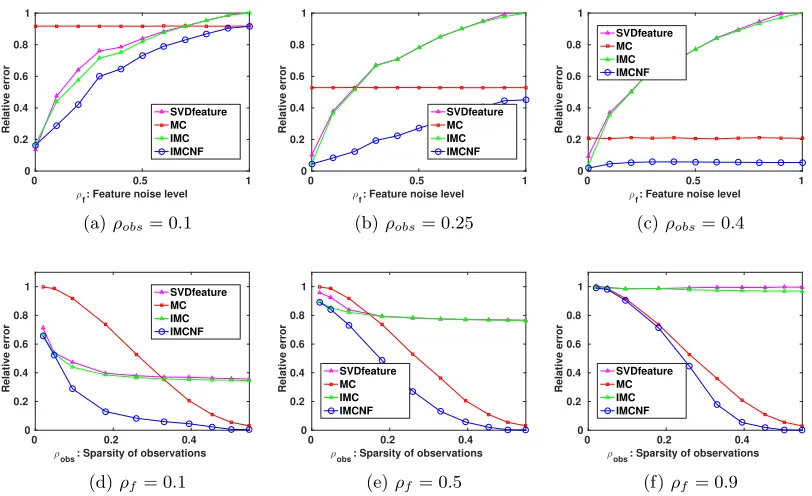
Figure 1: Performance of various methods for matrix completion under certain fixed sparsity of observationsρobs (upper figures) and fixed feature qualityρf (lower figures). We observe

that all feature-based methods perform better than standard matrix completion (MC) given perfect features (ρf = 0). However, IMCNF is less sensitive to feature noise asρf increases,

(18)

in X∗ (and Y∗) with bases orthogonal to X∗ (and Y∗). We then consider recovering the underlying matrix L0 given R,X and Y.

In this experiment, we consider the proposed IMCNF model (problem 6) which is an instance of the general problem (4) for exploiting noisy side information in matrix comple-tion case. We compare IMCNF with standard trace-norm regularized matrix complecomple-tion (MC), IMC (Jain and Dhillon, 2013) and SVDfeature (Chen et al., 2012). The recovered matrixL∗ from each algorithm is evaluated by the standard relative error:

kL∗−L0kF

kL0kF

. (11)

For each method, we select parameters from the set{10α_}2

α=−3 and report the one with the

best recovery. All results are averaged over 5 random trials.

Figure 1 shows results of each method under different ρobs = 0.1,0.25,0.4 and ρf =

0.1,0.5,0.9. We can first observe in upper figures that IMC and SVDfeature perform sim-ilarly under each ρobs, and moreover, their performance mainly depends on feature quality

and will not be affected much by the number of observations. Although their performance is comparable to IMCNF given perfect features (ρf = 0), their performance quickly drops

when features become noisy. This phenomenon is more clear in figure 1c and 1f where we see that given noisy features, IMC and SVDfeature will be easily trapped by feature noise and perform even worse than pure MC. Another interesting finding is that even if feature quality is as good as ρf = 0.1 (Figure 1d), IMC (and SVDfeature) still fails to achieve 0

relative error as the number of observations increases, suggesting that IMC is sensitive to feature noise and cannot guarantee recoverability when features are not perfect. On the other hand, we see that performance of IMCNF can be improved by both better features and more observations. In particular, it makes use of informative features to achieve lower error compared to MC and is also less sensitive to feature noise compared to IMC and SVDfeature. These results empirically support the analysis presented in Section 3.

4.1.2. Experiments on Robust PCA Setting

In this experiment, we examine the effect of both perfect and noisy side information in the proposed model for robust PCA as follows. We create a low-rank matrix L0 =U VT, where U, V ∈ _Rn×40_, _U

ij, Vij ∼ N(0,1/n) with n = 200. We also form a sparse noise

matrixS0 where each entry will be a non-zero entry with probabilityρs, and each non-zero

entry will take values from {±1} with equal probability. We then construct noisy features

X, Y ∈ _Rn×50 _{with a noise parameter} _ρ

f using the same construction in the previous

experiment, i.e. features X/Y will only span 40×(1−ρf) true bases of U/V. We then

consider to recover the low-rank matrix given the fully observed matrixR =L0+S0 along with noisy side informationX and Y.

(19)

0 0.5 1

ρ

f (feature noise level)

0 0.2 0.4 0.6 0.8 1

relative error

PCP PCPF PCPNF

(a)ρs= 0.1

0 0.5 1

ρ

0 0.2 0.4 0.6 0.8 1

relative error

PCP PCPF PCPNF

(b)ρs= 0.2

0 0.5 1

ρ

0 0.2 0.4 0.6 0.8 1

relative error PCP

PCPF PCPNF

(c)ρs= 0.3

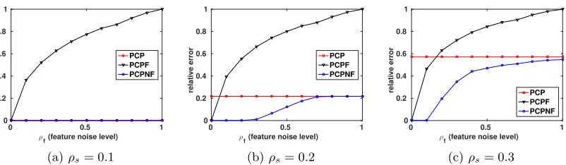
Figure 2: Performance of various methods for robust PCA given different feature noise level

ρf and sparsity of corruption ρs. These results show that PCPNF can make use of noisy

yet informative features for better recovery.

Figure 2 shows the performance of each method given different feature quality under

ρs = 0.1,0.2,0.3. We first see that when features are perfect (ρf = 0), both PCPF and

PCPNF can exactly recover the underlying matrix, while pure PCP fails to recover L0 if

ρs ≥0.2. This result confirms that both PCPNF and PCPF can leverage perfect features for

better recovery. However, as features become noisy (larger ρf), we see that PCPF quickly

performs worse as it is misled by noise in features, while PCPNF can better exploit noisy features for recovery. In particular, in Figure 2b, we observe that PCPNF still recovers L0

given noisy yet reasonably good features (0< ρf < 0.4), whereas PCP and PCPF fail to

recoverL0. These results show that PCPNF can take advantage of noisy side information for learning L0 given corrupted observations.

4.1.3. Experiments on Learning with Missing and Corrupted Observations

We now further examine to what extent can side information help the learning using our model when observations are both missing and corrupted. We consider the same construc-tion of L0 and S0 as in the previous experiment, and generate perfect feature matrices X, Y ∈Rn×dwithd=r+ 10. We then form the observation set Ωobs by randomly sampling

ρobs of entries from all n2 indexes, and take R =PΩobs(L0+S0) as the observed matrix.

The goal is therefore to recoverL0 given R along with side informationX and Y.

To exploit the advantage of side information, we consider the proposed model in form (5) where we further setα = 1 and β=∞ to forceN∗ to be zero for better exploiting perfect features, and compare it with the problem (1) which tries to recoverL0 only using structural

information. Notice that whenρobs = 1.0, the given problem becomes a robust PCA problem

whereR is a fully observed matrix, in which case problem (1) reduces to PCP method and our model reduces to PCPF objective (problem 8), respectively. From this aspect, we refer to problem (1) as “PCP with partial observations” (PCP-part) and our model as “PCPF with partial observations” (PCPF-part). The relative error criterion (11) is again used to evaluate the recovered matrix. Here, we regard the recovery to be successful if the error is less than 10−4. The parameterλin both methods are set to be 1/√ρobsn.

(20)

0.1 0.2 0.3 0.4 0.5 r/n

0.1 0.2 0.3 0.4

ρ

s

(a)ρobs= 1.0

0.1 0.2 0.3 0.4 0.5 r/n

0.1 0.2 0.3 0.4

ρ

s

(b)ρobs= 0.7

0.1 0.2 0.3 0.4 0.5 r/n

0.1 0.2 0.3 0.4

ρ

s

(c)ρobs= 0.5

Figure 3: Performance of PCP-part and PCPF-part with perfect features for recovering

L0 from missing and corrupted observations (controlled byρobs and ρs respectively). Both

methods achieve recovery in white region and fail in black region, yet there is a gray region where only PCPF-part achieves recovery. This shows that by leveraging perfect features, PCPF-part can recover a much larger class of L0 given both missing and corrupted

obser-vations are present.

we apply both methods to obtain the estimated low-rank matrix L∗. We then mark the grid point (r, ρs) to be white if recovery is attained by both methods and black if both

fail. We also observe that in several cases recovery cannot be attained by PCP-part but can be attained by PCPF-part, and these grid points are marked as gray. The results are shown in Figure 3. We observe that for each ρobs, there exists a substantial gray region

where matrices in such a region can be recovered only by PCPF-part. This result shows that in the case where both missing and corrupted entries are present, by exploiting side information, the proposed model is able to further recover a large amount of matrices which cannot be recovered if no side information is provided.

4.2. Real-world Applications

We now consider three applications—relationship prediction in signed networks, semi-supervised clustering and noisy image classification—which can be cast to problems of low-rank matrix learning from missing/corrupted entries with additional side information. As a consequence, we show that by learning the low-rank modeling matrix using our pro-posed model, we can achieve better performance compared to other methods for these applications as our model can better exploit side information in learning.

4.2.1. Relationship Prediction in Signed Networks

We first consider relationship prediction problem in an online review website Epin-ions (Massa and Avesani, 2006), where people can write product reviews and choose to trust or distrust others based on their reviews. Such a social network can be modeled as

a signed networkwhere each person is treated as an entity and trust/distrust relationships

(21)

Method IMCNF IMC MF-ALS HOC-3 HOC-5 Accuracy 0.9474±0.0009 0.9139±0.0016 0.9412±0.0011 0.9242±0.0010 0.9297±0.0011

AUC 0.9506 0.9109 0.9020 0.9432 0.9480

Table 2: Relationship prediction on Epinions network. We see that given noisy user features, IMC performs worse even than methods without features (MF-ALS and HOCs), while IMCNF outperforms others by successfully exploiting noisy features.

are proposed, a state-of-the-art approach is the low-rank model (Hsieh et al., 2012; Chiang et al., 2014) which first conducts matrix completion on the adjacency matrix and then uses the sign of the completed matrix for prediction. However, these methods are developed based only on network structure. Therefore, if features of users are available, we can also extend the low-rank model by incorporating user features in the completion step.

The experiment setup is described as follows. In this data set, there are aboutn= 105K users and m = 807K observed relationship pairs where 15% relationships are distrust. In addition to the who-trust-to-whom information, we are also given a user feature matrix

Z ∈ _Rn×41 _{where for each user a 41-dimensional feature is collected based on the user’s}

review history, such as number of positive/negative reviews the user gave or received. We consider the following prediction methods: walk and cycle-based methods including HOC-3 and HOC-5 (Chiang et al., 2014), and the original low-rank model with matrix factorization for the completion step (LR-ALS) (Hsieh et al., 2012). These methods make the prediction based on network structure without considering user features. We further consider the extended low-rank model where the completion step is replaced by IMCNF and IMC (Jain et al., 2013), both of which thus incorporate user features implicitly for prediction. Since row and column entities are both users, X = Y = Z is set for both IMCNF and IMC methods. We randomly divide the edges of the network into 10 folds and conduct the experiment using 10-fold cross validation, in which 8 folds are used for training, one fold for validation and the other for testing. Parameters for validation in each method are chosen from the sett2

α=−3{10α,5×10α}.

The averaged accuracy and AUC of each method are reported in Table 2. We first ob-serve that IMC performs worse than LR-ALS even though IMC takes features into account. It is because these user features are only partially related to the relationship matrix, and IMC is misled by such noisy features. On the other hand, IMCNF performs the best among all prediction methods, as it performs slightly better than LR-ALS in terms of accuracy and much better in terms of AUC. This result shows that IMCNF can exploit weakly informative features to make better prediction without being trapped by feature noise.

4.2.2. Semi-supervised Clustering

Semi-supervised clustering is another application which can be translated to learning a low-rank matrix with partial observations. Given a feature matrix Z ∈_Rn×d_of _n_{items and} _m

pairwise constraints specifying whether itemiand j are similar or dissimilar, the goal is to find a clustering of items such that most similar items are within the same cluster.

(22)

obtain a clustering purely from the pairwise constraints using matrix completion as follows. Let S ∈Rn×n be the (signed) similarity matrix constructed from the constraint set where Sij = 1 if item i and j are similar, −1 if dissimilar and 0 if similarity is unknown. Then

finding a clustering ofnitems becomes equivalent to finding a clustering on the signed graph

S, where the goal is to put items (denoted as nodes) intokgroups so that most edges within the same group are positive and most edges between groups are negative (Chiang et al., 2014). As a result, one can apply a matrix completion approach proposed in Chiang et al. (2014) to solve the signed graph clustering problem, which first conducts matrix completion on S and runs k-means on the top-k eigenvectors of completed S to obtain a clustering of nodes.

Apparently, either dropping features or constraint set is not optimal for semi-supervised clustering problem. Thus, many algorithms are proposed to take both item features and constraints into account, such as metric-learning-based approaches (Davis et al., 2007), spectral kernel learning (Li and Liu, 2009) and MCCC algorithm (Yi et al., 2013). Among many of them, MCCC algorithm is a cutting edge approach which essentially solves semi-supervised clustering using IMC objective. Observing that each pairwise constraint can be viewed as a sampled entry from the matrix L0 =U UT where U ∈ Rn×k is the clustering

membership matrix, MCCC tries to complete L0 back as ZM ZT using IMC objective. Furthermore, since the completed matrix is ideally L0 whose subspace spans U, it thus

conductsk-means on the top-keigenvectors of the completed matrix to obtain a clustering. However, since MCCC is based on IMC, its performance thus heavily depends on the quality of features. Therefore, we propose to replace IMC with IMCNF in the matrix completion step of MCCC, and then runk-means on the top-keigenvectors of the completed matrix to obtain a clustering. Both X and Y are again set to beZ as the target low-rank matrix describes the similarity between items. This algorithm can be viewed as an improved version of MCCC to handle noisy features Z.

We now compare our algorithm with k-means, signed graph clustering with matrix completion (Chiang et al., 2014) (SignMC) and MCCC (Yi et al., 2013) on three real-world data sets: Mushrooms, Segment and Covtype. 5 All of them are classification benchmarks where features and ground-truth labels of items are both available, and the ground-truth cluster of each item is defined by its ground-truth label. The statistics of data sets are summarized in Table 3. For each data set, we randomly samplem= [1,5,10,15,20,25,30]×

n clean pairwise constraints and input both constraints and features to each algorithm to obtain a clustering π, whereπi is the cluster index of itemi. We then evaluate π using the

following pairwise error:

n(n−1) 2

X

(i,j):π∗ i=πj∗

1[πi6=πj] + X

(i,j):π∗ i6=π∗j

1[πi =πj]

whereπ∗_i is the ground-truth cluster of itemi.

Figure 4 shows the clustering result of each method given various numbers of constraints on each data set. We first see that for the Mushrooms data set where features are perfect (100% training accuracy can be attained by a linear-SVM for classification), both MCCC

(23)

number of itemsn feature dimensiond number of clusters k

Mushrooms 8124 112 2

Segment 2319 19 7

Covtype 11455 54 7

Table 3: Statistics of semi-supervised clustering data sets.

0 0.5 1 1.5 2

x 105

0 0.1 0.2 0.3 0.4 0.5

Mushrooms

Number of observed pairs

Pairwise error

K−means SignMC MCCC IMCNF

0 1 2 3 4 5 6

x 104 0

0.1 0.2 0.3 0.4 0.5

Segment

Pairwise error

0 0.5 1 1.5 2 2.5 3

x 105 0

0.1 0.2 0.3 0.4 0.5

Covtype

Pairwise error

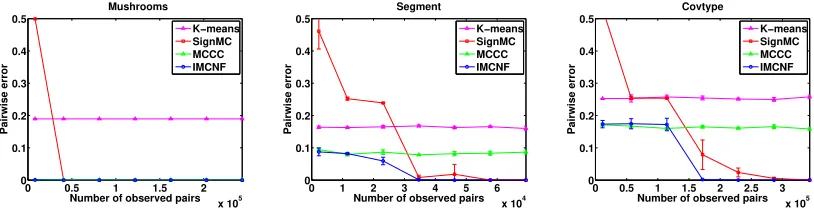
Figure 4: Performance of various semi-supervised clustering methods on real-world data sets. For the Mushrooms data set where features are perfect, both MCCC and IMCNF can output the ground-truth clustering with 0 error rate. For Segment and Covtype where features are more noisy, IMCNF model outperforms MCCC as its error decreases given more constraints.

and IMCNF can obtain the ground-truth clustering with 0 error rate, which indicates that MCCC (and IMC) is indeed effective with perfect features. For the Segment and Covtype data sets, we observe that the performance ofk-means and MCCC is dominated by feature quality. Although MCCC is still benefited from constraint information as it outperforms

k-means, it clearly does not make the best use of constraints since its performance is not improved even if number of constraints increases. On the other hand, the error rate of SignMC can always decrease down to 0 by increasing m; however, since it disregards fea-tures, it suffers from a much higher error rate than other methods when constraints are few. Finally, we see that IMCNF combines advantages from both MCCC and SignMC, as it not only makes use of features when few constraints are observed, but also leverages constraint information to avoid being trapped by feature noise. Therefore, the experiment shows that by carefully handling side information using IMCNF model, we can further improve the state-of-the-art semi-supervised clustering algorithm.

4.2.3. Noisy Image Classification

(24)

linear SVM classifiers kernel SVM classifiers

ρs Clean Noisy PCP PCPF ρs Clean Noisy PCP PCPF

0.1

91.96

59.63 86.33 87.88 0.1

98.33

18.47 94.85 95.89

0.2 38.16 85.94 87.48 0.2 10.32 94.55 95.48

0.3 25.63 78.52 79.84 0.3 10.32 87.00 87.78

Table 4: Digit classification accuracy of PCP and PCPF with Eigendigit features. The column Clean shows the accuracy on L0 and the column Noisy shows the accuracy on R. Denoised images from both PCP and PCPF achieve much higher accuracy than noisy images, and PCPF further outperforms PCP by incorporating Eigendigit features.

general human faces—known as Eigenface (Turk and Pentland, 1991)—could be used as features, and such features could be helpful in the denoising process.

Motivated by the above realization, here we consider multiclass classification on a set of noisy images from the MNIST data set. The data set includes 50,000 training images and 10,000 testing images, and each image is a 28×28 handwritten digit represented as a 784-dimensional vector. We first pre-train both multiclass linear and kernel SVM classifiers on the clean training images, and perturb the testing image set to generate noisy images

R. Precisely, let L0 ∈ R784×10000 be the set of (clean) testing images, where each row

denotes a pixel and each column denotes an image. We then construct a sparse noise matrixS0 ∈R784×10000 where ρs of entries are randomly picked to be corrupted by setting

their values to be 255. The observed noisy images is thus given by R= min(L0+S0,255).

In the following, we show that by exploiting features of row and column entities in this problem, we can better denoise the noisy images for classification.

Exploiting Eigendigit Features. We first exploit “Eigendigit” features to help denois-ing. We take the training image set to produce the Eigendigit features X∈R784×300 using

PCA and simply setY =I as we do not consider any column features here. We then input

R into PCP to derive a set of denoised images L∗_pcp and input R, X and Y (which is I) into PCPF (problem 8) to derive another set of denoised imagesL∗_pcpf =XM∗. Both L∗_pcp

and L∗_pcpf will be low rank approximations of the clean images. Note that although the Eigendigit features X will not satisfy (2) which is assumed in the derivation of PCPF, we could heuristically incorporate it using PCPF in this circumstance because X is still ex-pected to contain unbiased information of the low-rank approximation of the clean digits.6 To compare the quality of denoised images of PCP and PCPF, we input L∗_pcp and

L∗_pcpf to pre-trained SVMs for digit classification and report the results in Table 4. Both methods are somehow effective for denoising sparse noise, since accuracies achieved by the denoised images are much closer to the clean images compared to the noisy images. Furthermore, PCPF consistently achieves better accuracies than PCP under different ρs,

showing that incorporating Eigendigit features using PCPF is helpful on denoising process for classification.

Exploiting both Eigendigit and Label-relevant Features In addition to the Eigendigit features X, now we further exploit features for column entities. Ideally, the

(25)

0 0.5 1

ρ

f (noise level of Y) 70 75 80 85 90 95 100 Accuracy PCP PCPF PCPF-w/Y PCPNF-w/Y

(a) Linear SVM,ρs= 0.1

0 0.5 1

ρ

(b) Linear SVM,ρs= 0.2

0 0.5 1

ρ

(c) Linear SVM,ρs= 0.3

0 0.5 1

ρ

(d) Kernel SVM,ρs= 0.1

0 0.5 1

ρ

(e) Kernel SVM,ρs= 0.2

0 0.5 1

ρ

(f) Kernel SVM,ρs= 0.3

Figure 5: Digit classification accuracy of various methods with both Eigendigit and label-relevant features. For each ρs, we construct the label-relevant features Y with different

quality by varying ρf. The results show that PCPNF-w/Y is able to better exploit noisy

label-relevant features Y.

column featuresY may describe the relevant information between images, which could be extremely useful for classification. Thus, we generate the “label-relevant” features Y for column entities as follows. Let Y∗ ∈ R10000×10 be a perfect column feature matrix where

the i-th column of Y∗ is the indicator vector of digit i−1 (so Y∗ contains ground-truth label information). We then randomly pickρf of rows inY∗ and shuffle these rows to form

˜

Y, which correspondingly means that 10,000×ρf images have noisy relevant information

in ˜Y. Finally, we form the column featureY ∈R10000×50which spans ˜Y. Thus, the quality

of Y depends on the parameter ρf ∈ [0,1] and smaller ρf results in better label-relevant

features.

We consider four approaches for denoising in the following experiment. The first two baseline methods are PCP and PCPF with only Eigendigit features X. Both methods are the ones we considered in the previous experiment which do not take label-relevant features into account. Moreover, we consider using PCPF and PCPNF to incorporate both the Eigendigit featuresX and the label-relevant featuresY for denoising, and we name them as “PCPF-w/Y” and “PCPNF-w/Y” to emphasize that they embed the label-relevant features

Y. We apply each method to denoise noisy images under different ρf and ρs and examine

the quality of denoised images by testing the accuracies they achieve in pre-trained SVMs. The results are shown in Figure 5. In each figure, we fix the sparsity of noiseρsand try