Gap Safe Screening Rules for Sparsity Enforcing Penalties

Gap Safe Screening Rules for Sparsity Enforcing Penalties

Eugene Ndiaye [email protected]

LTCI, T´el´ecom ParisTech, Universit´e Paris-Saclay, 75013, Paris, France

Olivier Fercoq [email protected]

LTCI, T´el´ecom ParisTech, Universit´e Paris-Saclay, 75013, Paris, France

Alexandre Gramfort [email protected]

Inria, Universit´e Paris-Saclay, 91120, Palaiseau, France

LTCI, T´el´ecom ParisTech, Universit´e Paris-Saclay, 75013, Paris, France

Joseph Salmon [email protected]

LTCI, T´el´ecom ParisTech, Universit´e Paris-Saclay, 75013, Paris, France

Editor:David Wipf

Abstract

In high dimensional regression settings, sparsity enforcing penalties have proved useful to regularize the data-fitting term. A recently introduced technique calledscreening rules pro-pose to ignore some variables in the optimization leveraging the expected sparsity of the solutions and consequently leading to faster solvers. When the procedure is guaranteed not to discard variables wrongly the rules are said to besafe. In this work, we propose a uni-fying framework for generalized linear models regularized with standard sparsity enforcing penalties such as`1 or`1{`2norms. Our technique allows to discard safely more variables

than previously considered safe rules, particularly for low regularization parameters. Our proposed Gap Safe rules (so called because they rely on duality gap computation) can cope with any iterative solver but are particularly well suited to (block) coordinate descent methods. Applied to many standard learning tasks, Lasso, Sparse-Group Lasso, multi-task Lasso, binary and multinomial logistic regression, etc., we report significant speed-ups compared to previously proposed safe rules on all tested data sets.

Keywords: Convex optimization, screening rules, Lasso, multi-task Lasso, sparse logistic regression, Sparse-Group Lasso

1. Introduction

The computational burden of solving high dimensional regularized regression problem has led to a vast literature on improving algorithmic solvers in the last two decades. With the increasing popularity of`1-type regularization ranging from the Lasso (Tibshirani, 1996) or group-Lasso (Yuan and Lin, 2006) to regularized logistic regression and multi-task learning, many algorithmic methods have emerged to solve the associated optimization problems (Koh et al., 2007; Bach et al., 2012). Although for the simple`1 regularized least square a specific algorithm (e.g., the LARS (Efron et al., 2004)) can be considered, for more general formu-lations, penalties, and possibly larger dimensions, (block) coordinate descent has proved to be an efficient strategy (Friedman et al., 2010).

c

Our main objective in this work is to propose a technique that can speed-up any iterative solver for such learning problems, and that is particularly well suited for (block) coordinate descent method as this type of method can easily ignore useless coordinates1.

The safe rules introduced by El Ghaoui et al. (2012) for generalized `1 regularized problems, is a set of rules allowing to eliminate features whose associated coefficients are guaranteed to be zero at the optimum, even before starting any algorithm. Relaxing the safe rule, one can obtain some additional speed-up at the price of possible mistakes. Such heuristic strategies, calledstrong rules by Tibshirani et al. (2012) reduce the computational cost using an active set strategy, but require multiple post-processing to check for features possibly wrongly discarded.

Another road to speed-up screening method has been pursued following the introduction ofsequential safe rules (El Ghaoui et al., 2012; Wang et al., 2012; Xiang et al., 2014; Wang et al., 2014). The idea is to improve the screening thanks to the computation done for a previous regularization parameter as in homotopy/continuation methods. This scenario is particularly relevant in machine learning, where one computes solutions over a grid of regularization parameters, so as to select the best one, e.g., by cross-validation. Never-theless, the aforementioned methods suffer from the same problem as strong rules, since relevant features can be wrongly disregarded. Indeed, sequential rules usually rely on the exact knowledge of certain theoretical quantities that are only known approximately. Es-pecially, for such rules to work one needs the exact dual optimal solution from the previous regularization parameter, a quantity (almost) never available to the practitioner.

The recent introduction ofdynamic safe rulesby Bonnefoy et al. (2015, 2014) has opened a new promising venue by performing variable screening, not only before the algorithm starts, but also along the iterations. This screening strategy can be applied for any standard optimization algorithm such as FISTA (Beck and Teboulle, 2009), primal-dual (Chambolle and Pock, 2011), augmented Lagrangian (Boyd et al., 2011). Yet, it is particularly relevant for strategies that can benefit from support reduction or active sets (Kowalski et al., 2011; Johnson and Guestrin, 2015), such as coordinate-descent (Fu, 1998; Friedman et al., 2007, 2010).

This paper contains a synthesis and a unified presentation of the methods introduced first for the Lasso in (Fercoq et al., 2015) and then for`1{`2 norms in (Ndiaye et al., 2015) as well as for Sparse-Group Lasso in (Ndiaye et al., 2016b). Our so-called Gap Safe rules (because the screening rules rely on duality gap computations), improved on dynamic safe rules for a broad class of learning problems with the following benefits:

• Gap Safe rules are easy to insert in existing solvers,

• they are proved to be safe and unify sequential and dynamic rules,

• they lead to improved speed-ups in practice w.r.t. previously known safe rules,

• they achieve fast variable identifications2.

1. By construction a method like LARS (Efron et al., 2004), that applies only to the Lasso case, cannot beneficiate from screening rules.

Furthermore, it is worth noting that strategies also leveraging dual gap computations have recently been considered to safely discard irrelevant coordinates: Shibagaki et al. (2016) have considered screening rules for learning tasks with both feature sparsity and sample sparsity, such as for `1-regularized SVM. In this case, some interesting developments have been proposed, namelysafe keeping strategies, which allow to identify features and samples that are guaranteed to be active. Constrained convex problems such as minimum enclosing ball can also be included as shown in Raj et al. (2016). The Blitz algorithm by Johnson and Guestrin (2015) aims to speed up working set methods using duality gaps computations; significant gains were also obtained in limited-memory and distributed settings.

We introduce the general framework of Gap Safe screening rules in Section 3; in Section 4 we instantiate them on various strategies including static, dynamic and sequential ones, and show how the Gap Safe methodology can encompass all of them. The converging nature of the Gap Safe rules is also discussed. In Section 5, we investigate the specific form of our rules for standard machine learning models: Lasso, Group Lasso, Sparse-Group Lasso, logistic regression with `1 regularization, etc. Section 6 reports a comprehensive set of experiments on four different learning problems using either dense or sparse data. Results demonstrate the systematic gain in computation time of the Gap Safe rules.

2. Notation and Background on Optimization

For any integerdPN, we denote byrdsthe sett1, . . . , duand byQJ_{the transpose of a matrix}

Q. Our observation vector isyPRnwherenrepresents the number of samples. The design matrix X “ rx1, . . . , xnsJ P Rnˆp has p explanatory variables (or features) column-wise, andnobservations row-wise. For a norm Ω, we writeBΩ the associated unit ball,k¨k2 is the `2 norm (andx¨,¨yfor the associated inner product),k¨k1 is the`1 norm, andk¨k8 is the`8 norm. The`2 unit ball is denoted byB2 (or simplyB) and we writeBpθ, rqthe`2 ball with centerθand radiusr. For a vectorβ PRp, we denote by supppβq the support ofβ (i.e.,the set of indices corresponding to non-zero coefficients) and by kBk2

F “ řp

j“1

řq

k“1B2j,k the

Frobenius norm of a matrix BPRpˆq. We denoteptq` “maxp0, tqand ΠCp¨qthe projection operator over a closed convex setC. The soft-thresholding operator STτ (at levelτ ě0) is

defined for anyxPRd by rSTτpxqsj “signpxjqp|xj| ´τq`.

The parameter to recover is a vector β “ pβ1, . . . , βpqJ admitting a group structure. A

group of features is a subsetgĂ rpsand ng is its cardinality. The set of groups is denoted

by G and we focus only on non-overlapping groups3 that form a partition of the set rps. We denote by βg the vector in Rng which is the restriction of β to the indices in g. We write rβgsj the j-th coordinate ofβg. We also use the notationXg PRnˆng to refer to the sub-matrix of X assembled from the columns with indices j Pg and Xj when the groups

are a single feature,i.e., wheng“ tju.

Some elements of convex analysis used in the following sections are introduced here. For a function f :Rd Ñ r´8,`8s, the Fenchel-Legendre transform4 of f, is the function f˚ _:

Rd Ñ r´8,`8s defined by f˚_{puq “ sup}

zPRdxz, uy ´fpzq. The sub-differential of

a function f at a point x is denoted by Bfpxq. For a norm Ω over Rd, its dual norm is written ΩD _{and is defined for any u P}

Rd by ΩDpuq “ maxΩpzqď1xz, uy. Note that in

the case of a group-decomposable norm, one can check that ΩDpβq “maxgPGΩDgpβgq and

BΩpβq “ΠgPGBΩgpβgq.

We remind below useful standard results from convex analysis:

Proposition 1 (Fermat’s Rule) (see (Bauschke and Combettes, 2011, Proposition 26.1) for a more general result) For any convex function f :RdÑR:

x‹

Parg min

xPRd

fpxq ðñ0P Bfpx‹_{q. (1)}

Proposition 2 (Subdifferential of a Norm) (see (Bach et al., 2012, Proposition 1.2)) The sub-differential of the norm Ω at x, is given by

BΩpxq “

#

tzPRd: ΩDpzq ď1u “BΩD, if x“0,

tzPRd: ΩDpzq “1 and zJx“Ωpxqu, otherwise. (2)

3. Gap Safe Framework

We propose to estimate the vector of parametersβ by solving

ˆ βpλq

Parg min

βPRp

Pλpβq, forPλpβq:“Fpβq `λΩpβq:“ n ÿ

i“1

fipxJi βq `λΩpβq , (3)

where all fi : R ÞÑ R are convex and differentiable functions with 1{γ-Lipschitz gradient and Ω :Rp ÞÑ R` is a norm that is group-decomposable, i.e., Ωpβq “ř_gPGΩgpβgq where

each Ωg is a norm on Rng. The λ parameter is a non-negative constant controlling the trade-off between the data fitting term and the regularization term. Popular instantiations of problems of the form (3) are detailed in Section 5.

Theorem 3 A dual formulation of the optimization problem defined in (3)is given by

ˆ

θpλq“arg max

θP∆X ´

n ÿ

i“1

f_i˚p´λθiq “:Dλpθq, (4)

where ∆X “ tθPRn:@gPG,ΩD_g pXJ

g θq ď1u. Moreover, the Fermat’s rule reads:

@iP rns, θˆp_iλq “ ´∇fipxJi βˆpλqq{λ plink equationq, (5)

@gPG, X_gJθˆpλq P BΩgpβˆgpλqq psub-differential inclusionq. (6)

For any θ P Rn let us introduce Gpθq :“ r∇f1pθ1q, . . . ,∇fnpθnqsJ P Rn. Then the pri-mal/dual link equation can be written ˆθpλq_{“ ´GpXβˆ}pλq_{q{λ .}

3.1 Safe Screening Rules

Following the seminal work by El Ghaoui et al. (2012) screening techniques have emerged as a way to exploit the known sparsity of the solution by discarding features prior to starting a sparse solver. Such techniques are referred to in the literature as safe rules when they screen out coefficients guaranteed to be zero in the targeted optimal solution. Zeroing those coefficients allows to focus exclusively on the non-zero ones (likely to represent signal) and helps reducing the computational burden.

One well known extreme is the following: forλą0 large enough, 0 is the unique solution of (3). Indeed,

0Parg min

βPRp

Fpβq `λΩpβqðñ(1) 0P t∇Fp0qu `λBΩp0qðñ(2) ΩDp∇Fp0qq ďλ.

Hence we recall the first “naive” screening rule, stating that for large values of the regular-ization parameter, all features can be discarded.

Proposition 4 (Critical Parameter: λmax) For any λą0, 0Parg min

βPRp

Pλpβq ðñλěλmax:“ΩDp∇Fp0qq “ΩDpXJGp0qq .

So from now on, we will only focus on the case whereλăλmax. In this case, screening rules rely on a direct consequence of Fermat’s rule (6). If ˆβgpλq ‰0, then ΩDgpXgJθˆpλqq “1 thanks

to Equation (2). Since ˆθpλq_P∆

X, it implies, by contrapositive, that if ΩDgpXgJθˆpλqq ă1 then

ˆ

βgpλq “0. This relation means that theg-th group can be discarded whenever ΩgDpXgJθˆpλqq ă

1. However, since ˆθpλq_{isunknown— unlessλąλ}

max, in which case ˆθpλq“Gp0q{λ— this rule is of limited use. Fortunately, it is often possible to construct a set RĂRn, called a

safe region, that contains ˆθpλq_{. This observation leads to the following result.}

Proposition 5 (Safe Screening Rule El Ghaoui et al. (2012)) If θˆpλq

P R, and g P

G:

max

θPRΩ D

g pXgJθq ă1ùñΩDgpXgJθˆpλqq ă1ùñβˆgpλq“0 . (7)

The so-calledsafe screening rule consists in removing theg-th group from the problem whenever the previous test is satisfied, since then ˆβgpλq is guaranteed to be zero. Should R

be small enough to screen many groups, one can observe considerable speed-ups in practice as long as the testing can be performed efficiently. A natural goal is to find safe regions as narrow as possible: smaller safe regions can only increase the number of screened out variables. To have useful screening procedures one needs:

• the safe region Rto be as small as possible (and to contain ˆθpλq_),

• the computation of the quantity max

θPR Ω D

gpXgJθq to be cheap.

3.2 Gap Safe Regions

Various shapes have been considered in practice for the safe region R such as balls (El Ghaoui et al., 2012), domes (Fercoq et al., 2015) or more refined sets (see Xiang et al. (2014) for a survey). Here we consider for simplicity the so-called “sphere regions” (following the terminology introduced by El Ghaoui et al. (2012)) choosing a ball R “Bpθ, rq as a safe region. Thanks to the triangle inequality, we have:

max

θPBpθ,rq

ΩD_gpXJ

gθq ďΩDg pXgJθq ` max θPBpθ,rq

ΩD_gpXJ

gpθ´θqq,

and denoting ΩD_gpXgq:“supu‰0 ΩD

gpXgJuq

kuk₂ the operator norm of Xg associated to ΩDgp¨q, we

deduce from Proposition 7 the screening rule for theg-th group:

Safe sphere test: If ΩD_gpX_gJθq `rΩD_gpXgq ă1, then βˆgpλq“0 . (8)

3.2.1 Finding a Center

To create a useful center for a safe sphere, one needs to be able to create dual feasible points, i.e., points in the dual feasible set ∆X. One such point is θmax :“ ´Gp0q{λmax

which leads to the original static safe rules proposed by El Ghaoui et al. (2012). Yet, it has a limited interest, being helpful only for a small range of (large) regularization parameters λ, as discussed in Section 4.1. A more generic way of creating a dual point that will be key for creating our safe rules is to rescale any point zPRn such that it is in the dual set ∆X.

The rescaled point is denoted by Θpzq and is defined by

Θpzq:“

#

z, if ΩDpXJ_{zq ď1,} z

ΩD_pXJ_zq, otherwise.

(9)

This choice guarantees that@zPRn,Θpzq P∆X. A candidate often considered for

comput-ing a dual point is the (generalized) residual termz“ ´GpXβq{λ. This choice is motivated by the primal-dual link equation 5 i.e.,θˆpλq_{“ ´GpXβ}ˆpλq_q{λ.

3.2.2 Finding a Radius

Now that we have seen how to create a center candidate for the sphere, we need to find a proper radius, that would allow the associated sphere to be safe. The following theorem proposes a way to obtain a radius using the duality gap. The quantity

Gap_λpβ, θq:“Pλpβq ´Dλpθq (10)

is often referred to as the duality gap in the convex optimization literature, hence the name of our proposed Gap Safe framework. This quantity is also a useful tool when designing a stopping criterion: noting that for any β PRp, θ P∆X,Pλpβq ´Pλpβˆpλqq ďGapλpβ, θq, it

suffices to find a primal-dual pair with a duality gap smaller thanto ensure an -accuracy primal solution for Problem 3.

Theorem 6 (Gap Safe Sphere) Assuming thatF has 1{γ-Lipschitz gradient, we have

@βPRp,@θP∆X,

ˆ θpλq

´θ

2 ď

d

2Gap_λpβ, θq

Hence the set R“Bpθ,a2Gap_λpβ, θq{γλ2_{q is a safe region for anyβ PR}n _{and θ}

P∆X.

Proof Remember that @i P rns, fi is differentiable with a 1{γ-Lipschitz gradient. As

a consequence, @i P rns, f˚

i is γ-strongly convex (Hiriart-Urruty and Lemar´echal, 1993,

Theorem 4.2.2, p. 83) and so the dual function Dλ isγλ2-strongly concave:

@pθ1, θ2q PRnˆRn, Dλpθ2q ďDλpθ1q ` x∇Dλpθ1q, θ2´θ1y ´

γλ2

2 kθ1´θ2k 2 2 . Specifying the previous inequality for θ1“θˆpλq_{, θ2}

“θP∆X, one has

Dλpθq ďDλpθˆpλqq ` x∇Dλpθˆpλqq, θ´θˆpλqy ´

γλ2 2

ˆ θpλq´θ

2 2 . By definition, ˆθpλq _maximizesD

λ on ∆X, so, x∇Dλpθˆpλqq, θ´θˆpλqy ď0. This implies

Dλpθq ďDλpθˆpλqq ´

γλ2 2

ˆ θpλq

´θ

2 2.

By weak duality @β P Rp, Dλpθˆpλqq ď Pλpβq, hence @β P Rp,@θ P ∆X, Dλpθq ď Pλpβq ´ γλ2

2 kθˆ

pλq

´θk2

2 and the conclusion follows.

Remark 7 To build a Gap Safe region as in Equation (11), we only need strong convexity in the dual which is equivalent to smoothness of the loss function whereas the screening prop-erty (7), requires group separability of norms. Hence our framework of Gap Safe screening rule automatically applies for a large class of problems.

Remark 8 During the review process, we became aware of a possible improvement for the radius Johnson and Guestrin (2016). In the Blitz framework, their approach leads to a potentially smaller radius, using a strongly concave upper bound of the dual function whose maximum is known. In our framework, this can be used to improve the safe radius by a?2

factor in the static case. This is unclear to us whether this can be done for the sequential and dynamic version. For the SVM problem Zimmert et al. (2015) got the same improvement by writing the duality gap as a function of primal variables only.

3.2.3 Safe Active Set

Note that any time a safe rule is performed thanks to a safe region R “Bpθ, rq, one can associate a safe active set A_θ,r, consisting of the features that cannot be removed yet by the test in Equation (8). Hence, the safe active set contains the true support of ˆβpλq_.

Definition 9 (Safe Active Set) For a center θ P ∆X and a radius r ě 0, the safe

(sphere) active set consists of the variables not eliminated by the associated (sphere) safe rule, i.e.,

When choosing z “ ´GpXβq{λ as proposed in Section 3.2.1 as the current residual, the computation of θ “ Θpzq in Equation (9) involves the computation of ΩDpXJ_{zq. A} straightforward implementation would cost Opnpq operations. This can be avoided: when using a safe rule one knows that the index achieving the maximum for this norm is in

Apθ, rq. Indeed, by construction of the safe active set, it is easy to see that ΩDpXJ_{zq “} maxgPApθ,rqΩDgpXgJzq. In practice the evaluation of the dual gap is therefore Opnqq where

q is the size of Apθ, rq. In other words, using a safe screening rule also speeds up the evaluation of the stopping criterion.

3.3 Outline of the Algorithm

When designing a supervised learning algorithm with sparsity enforcing penalties, the tuning of the parameter λin Problem (3) is crucial and is usually done by cross-validation which requires evaluation over a grid of parameter values. A standard grid considered in the literature is λt “ λmax10´δt{pT´1q with a small δ, say δ “ 10´2 or 10´3, see for instance (B¨uhlmann and van de Geer, 2011)[2.12.1] or the glmnet package (Friedman et al., 2010). The parameterδ has an important influence on the computational burden: computing time tends to increase for smallλ, the primal iterates being less and less sparse, and the problem to solve more and more ill-posed. It is customary to start from the largest regularizer λ0“λmaxand then to perform iteratively the computation of ˆβpλtq after the one of ˆβpλt´1q. This leads to computing the models in the order of increasing complexity: this allows important speed-up by benefiting of warm start strategies.

Here we propose a simple pathwise algorithm divided in two step:

• Active warm start: improve solver initialization by solving the problem restricted to an initial estimation of the support based on sequential informations along the regularization path (see Section 4.4 for details on the various strategies investigated).

• Dynamic Gap Safe Screening: use the informations gained during the iterations of the algorithm to obtain a smaller safe region therefore a greater elimination of inactive variables (see Section 4.3).

We summarize our strategy for solving the problem given by Equation (3) in Algorithm 1 and 2. The notation Solverp. . .qrefers to any numerical solver that produces an approximation of the solution of (3) and SolverUpdatep. . .q is the updating scheme of the current vector along the iterations5. We consider solvers that can use a (primal) warm start point.

4. Screening strategies and theoretical analysis

We now describe the simplest safe rule strategy, which we refer to as the static strategy.

4.1 Static Safe Rules

The first static safe rule, introduced by El Ghaoui et al. (2012), discards variables before any computation thanks to Proposition 4. Here, the (safe) sphere is fixed once and for all,

Algorithm 1 Pathwise algorithm with active warm start Input : X, y, , K, fce, pλtqtPrT´1s

fortP rT´1sdo

β “βqpλt´1q and // Get previous -solution

Get an initial (safe or not) support estimator S“Spβqpλt´1qq

βS“SolverpXS, y, βS, , K, fce, λtq // Active warm start q

βpλtq_{“SolverpX, y, β, , K, f}ce_{, λ}

tq // Solve over all variables

Output: ´

q

βpλtq¯ tPrT´1s

Algorithm 2 Iterative solver with GAP safe rules: SolverpX, y, β, , K, fce, λq

Input : X, y, β, , K, fce_{, λ // Warm start is authorized here through β}

forkP rKsdo

if k mod fce“1then

Compute a dual variable θ“ ´GpXβq{maxpλ,ΩDpXJ_GpXβqqq Stop if Gap_λpβ, θq ď

r “

b

2Gap_λpβ,θq

γλ2 // Get Gap Safe radius as in Equation (11)

A“ gPG: ΩD_g pXJ

gθq `rΩDg pXgq ě1 (

// Get Safe active set as in Equation (12)

βA “SolverUpdatepXA, y, βA, λq // Solve on current Safe active set Output: βqpλq

hence the name static. The static rule reads:

Static sphere rule: If ΩD_g pX_gJθmaxq `rmaxΩDg pXgq ă1, then βˆgpλq“0 ,

Center: θmax:“ ´Gp0q{λmax ,

Radius: rmax:“a2Gap_λp0, θmaxq{γλ2 _.

There is a threshold λcritic such that for any λ smaller than λcritic the test from the Static sphere rule can never be satisfied. This phenomenon appears clearly in the numerical experiments presented in Section 6. In simple cases a closed form for λcritic can even be provided. For instance, in the case of the Group Lasso, El Ghaoui et al. (2012) proposed

to usermax“

1

λ ´

1

λmax

kyk2, and simple calculation gives:

λcritic:“λmaxˆmin

gPG

kyk₂ΩD gpXgq

λmax`kyk2ΩDgpXgq ´ΩDg pXgGp0qq

.

4.2 Sequential Safe Rules

Provided that the λ’s are close enough along the regularization parameters, knowing an estimate of ˆβpλt´1q _{gives a clever initialization to compute ˆβ}pλtq_{. To initialize the solver for} a newλt, a natural choice is to set the primal variable equal to ˇβpλt´1q, an approximation of

ˆ

one can reuse prior dual information to improve the screening as well (El Ghaoui et al., 2012). This leads to the sequential strategy to screen for a new λt:

Sequential sphere rule: If ΩD_g pX_gJθˇpλt´1q_{q `r}

tΩDgpXgq ă1, then βˆgpλtq“0 ,

Center: θˇpλt´1q _:

“Θp´GpXβˇpλt´1q_q{λ

t´1q , Radius: rt:“

b

2Gap_λtpβˇpλt´1q_,θˇpλt´1q_q{γλ2 t .

Remark 10 Previous works in the literature (Wang et al., 2012; Wang and Ye, 2014; Wang et al., 2014; Lee and Xing, 2014) proposed sequential safe rules, though they were generally used in an unsafe way in practice. Indeed, such rules relied on the exact knowledge of θˆpλt´1q _{to screen out coordinates of β}ˆpλtq_{. Unfortunately, it is impossible to obtain such}

a point6 since it is the solution of an optimization problem typically solved by an iterative solver, hence such it is only known up to a limited precision. By ignoring such inaccuracy in the knowledge ofθˆpλt´1q _{one can wrongly eliminate variables that do belong to the support}

of βˆpλtq_{. Without a posteriori checking the screened out features, this could prevent the} algorithm from converging, as shown in (Ndiaye et al., 2016b, Appendix B).

4.3 Dynamic Safe Rules

Another road to speed up solvers using screening rules was proposed by Bonnefoy et al. (2014, 2015) under the name “dynamic safe rules”. For a fixed λ, it consists in performing screening along with the iterations of the optimization algorithm used to solve Problem (3). Denoting bykthe iteration number, they introduced a rule for the Lasso that consists of a safe sphere with centery{λand radiusky{λ´θkk, where θk is a current dual feasible point.

Let us consider a sequencepβkqthat converges to a primal solution ˆβpλq. For creating a

dual feasible point, we apply the rescaling introduced in Equation (9) to z“ ´GpXβkq{λ

and the dynamic strategy can be summarized by

Dynamic sphere rule: If ΩD_g pXJ

gθkq `rkΩDgpXgq ă1, then βˆgpλq“0 ,

Center: θk :“Θp´GpXβkq{λq defined thanks to (9) ,

Radius: rk:“ a

2Gap_λpβk, θkq{γλ2 .

In practice the computation of the duality gap can be expensive due to the matrix vector operations needed to compute XJ_GpXβ

kq. For instance in the Lasso case, a dual

gap computation requires almost as much computation as a full pass of coordinate descent over the data. Hence, it is recommended to evaluate the dynamic (safe) rule only every few passes over the data set. In all our experiments, we have set this screening frequency parameter tofce _“10.

Note that contrary to the original dynamic screening rules proposed by Bonnefoy et al. (2014, 2015), the Gap Safe rules we introduced are converging in the sense that our safe regions converge to the singleton tθˆpλq_{u (see Section 4 for more details). Indeed, their} proposed safe sphere was centered ony{λ, and their radius can only be greater than ky{λ´ ˆ

θpλq_{k in the Lasso case they consider. We provide a visual comparison in Figure 1.}

(a) Bonnefoyet al.(2014) safe region (b) Gap Safe region

Figure 1: Illustration of safe region differences between Bonnefoy et al. (2014) and Gap Safe strategies for the Lasso case; note thatγ “1 in this case. Hereβ is a primal point, θ is a dual feasible point (the feasible region ∆X is in orange, while the

respective safe ballsR are in blue).

4.4 Active Warm Start

An another variant to further reduce running time in the active warm start, recently introduced by Ndiaye et al. (2016a) for speeding-up concomitant Lasso computations. Instead of simply leveraging the previous primal solution, the active warm start strat-egy also makes use of the previous safe active set Apθt´1, rt´1q, with θt´1 “ θˇpλt´1q and rt´1 “ rλt´1pβˇ

pλt´1q_,θˇpλt´1q_{q. The idea is to take as a new primal warm start point, the}

(approximate) minimizer ofPλt under the additional constraint that its support is included in the safe active setApθt´1, rt´1q i.e.,

r

βpλt´1,λtq

Parg min

βPRp

Fpβq `λtΩpβqs.t. supppβq ĎApθt´1, rt´1q . (13)

4.5 Theoretical Analysis

Dynamic safe screening rules have practical benefits since they increase the number of screened out variables as the algorithm proceeds. In this section, it is shown that Gap Safe rules allow to have sharper and sharper dual regions along the iterations, accelerating support identification. Before this, the following proposition states that if one relies on a primal converging algorithm, then the dual sequence we propose is also converging. Note that the convergence is maintained to the same primal solution when the primal solution is non-unique.

Proposition 11 (Convergence of the Dual Points) Let βk be a current estimate of

a primal solution βˆpλq _{and θ}

k “ Θp´GpXβkq{λq be the current estimate of θˆpλq. Then,

limkÑ`8βk“βˆpλq implies limkÑ`8θk“θˆpλq.

Proof Let αk“maxpλ,ΩDpXJGpXβkqqq, we have:

θk´

ˆ θpλq

2“

GpXβˆpλq_q

λ ´

GpXβkq

αk 2 ď ˇ ˇ ˇ ˇ 1 λ´ 1 αk ˇ ˇ ˇ ˇ

kGpXβkqk2`

GpX

ˆ βpλq

q ´GpXβkq

2

λ .

If βk Ñ βˆpλq, then αk Ñ maxpλ,ΩDpXJGpXβˆpλqqqq “ maxpλ, λΩDpXJθˆpλqqq “ λ since

GpXβˆpλq_{q “ ´λθ}ˆpλq_{thanks to the link-equation (5) and since ˆθ}pλq_{is feasible, Ω}D_pXJ_θˆpλq_{q ď 1.} Hence, both terms in the previous inequality converge to zero.

Let us now describe the notion of converging safe regions and converging safe rules introduced in (Fercoq et al., 2015, Definition 1).

Definition 12 Let pRkqkPN be a sequence of closed convex sets in R

n _{containing θˆ}pλq_{. It}

is a converging sequence of safe regions if the diameters of the sets converge to zero. The associated safe screening rules are referred to as converging.

When θk “Θp´GpXβkq{λq, Proposition 11 guarantees that Gap Safe spheres are

con-verging. Indeed, the sequence of radiusrk “ p2Gapλpβk, θkq{pγλ2qq1{2 converges to 0 with

kby strong duality, hence the sequence Bpθk, rkq converges totθˆpλquwhich means that the

proposed Gap Safe sphere is asymptotically optimal.

We now prove that one recovers a specific set, called the equicorrelation set in finite time with any converging strategy.

Definition 13 The equicorrelation set is defined asE_λ :“

!

gPG: ΩD_gpX_gJθˆpλqq “1 )

.

Indeed, the following proposition asserts that after a finite number of steps, the equicorre-lation set Eλ is exactly identified. Such a property is sometimes referred to as finite

Figure 2: Illustration of the inclusions between several remarkable sets: supppβq Ď

Apθ, rq Ď rps and supppβˆpλq

q Ď Eλ Ď Apθ, rq Ď rps, where β, θ is a primal/dual

pair.

Proposition 14 (Identification of the Equicorrelation Set)

For any sequence of converging safe active set pApθk, rkqqkPN, we have limkÑ8Apθk, rkq “

E_λ. More precisely, there exists an integer k0 PN such that Apθk, rkq “Eλ for all kěk0.

Proof We proceed by double inclusion. First remark that Eλ “ Apθˆpλq,ˆrλq where ˆrλ :“

2pPλpβˆpλqq ´Dλpθˆpλqqq{γλ2 “ 0 (thanks to strong duality), so for all k P N, we have

E_λĎApθk, rkq.

Reciprocally, suppose that there exists a non active group g P G i.e., ΩD

g pXgJθˆpλqq ă

1 that remains in the active set Apθk, rkq for all iterations i.e., @k P N,ΩDg pXgJθkq `

rkΩDgpXgq ě 1. Since limkÑ8θk “ θˆpλq and limkÑ8rk “ 0, we obtain ΩDg pXgJθˆpλqq ě 1

by passing to the limit. Hence, by contradiction, there exits an integer k0 P N such that

Ec

λĎApθk0, rk0q

c_.

4.6 Alternative Strategies: a Brief Survey

4.6.1 The Seminal Safe Regions

The first Safe Screening rules introduced by El Ghaoui et al. (2012) can be generalized to Problem (3) as follows. Take ˆθpλ0q _{the optimal solution of the dual problem (4) with a} regularization parameter λ0. Since ˆθpλq _{is optimal for problem (4) one obtains ˆθ}pλq _{P tθ :}

Dλpθq ěDλpθˆpλ0qqu. This set was proposed as a safe region by El Ghaoui et al. (2012).

In the regression case (where fipzq “ pyi ´zq2{2), it is straightforward to see that it

corresponds to the safe sphereBpy{λ,ky{λ´θˆpλ0q_k2q.

4.6.2 ST3 and Dynamic ST3

Following (7), the safe sphere test given by Equation (8) is more efficient when θ is near ˆ

A refined sphere rule can be obtained in the regression case by exploiting geometric informations in the dual space. This method was originally proposed in Xiang et al. (2011) and extended in Bonnefoy et al. (2014) with a dynamic refinement of the safe region.

Let g‹Parg maxgPGΩDg pXJyq(note that ΩDg‹pXJyq “λmax), and let us define

V‹ :“ tθPRn: ΩDg‹pXg‹Jθq ď1u andH‹ :“ tθPRn: ΩDg‹pXg‹Jθq “1u.

We assume that the dual norm is differentiable atXJ

g‹y{λmax(which is true in all the cases presented in Section 5). Let η :“ Xg‹∇ΩDg‹pX

J

g‹y{λmaxq be the vector normal to V‹ at

y{λmax and define

θ:“ΠH‹ ´y

λ

¯

“ y λ´

x_λy, ηy ´1

kηk2₂ η and rθ:“

c

y λ´θ

2 2´

y λ´θ

2 2 ,

where θ P ∆X is any dual feasible vector. Following the proof in (Ndiaye et al., 2016b,

Appendix D), one can show that ˆθpλq _{P Bpθ, r}

θq. The special case where θ “ y{λmax corresponds to the original ST3 introduced in Xiang et al. (2011) for the Lasso. A further improvement can be obtained by choosing dynamically θ “ θk along the iterations of an

algorithm, this strategy corresponding to DST3 introduced in Bonnefoy et al. (2014, 2015) for the Lasso and Group Lasso, and in Ndiaye et al. (2016b) for the Sparse-Group Lasso.

4.6.3 Dual Polytope Projection

In the regression case, Wang et al. (2012) explore other geometric properties of the dual solution. Their method is based on the non-expansiveness of projection operators7. Indeed, for ˆθpλq _{(resp. θˆ}pλ0q_{q) being optimal dual solution of (4) with parameter λ (resp. λ0),} one has: kθˆpλq_´θˆpλ0q_k

2 “ kΠ∆Xpy{λq ´Π∆Xpy{λ0qk2 ď ky{λ´y{λ0k2 and hence ˆθpλq P

Bpθˆpλ0q_{,ky{λ´y{λ0k2q. Unfortunately, those regions are intractable since they required the}

exact knowledge of the optimal solution ˆθpλ0q _{which is not available in practice (except for} λ0“λmax). It may lead to un-safe screening rules as discussed in Remark 10.

Remark 15 The preceding spheres are mainly based on the fact that θˆpλq _{“ Π}

∆Xpy{λq which is limited to the regression case. Thus, those methods are not appropriate for more general data fitting term which greatly reduces the scope of such rules.

Remark 16 The radius of the regions above do not converge to zero even in the dynamic case (DST3), and the (fixed) center of the preceding sphere can be far from θˆpλq _whenλgets

small. Thus, those regions are not converging and are irrelevant for dynamic screening.

4.6.4 Strong rules

The Strong rules were introduced in Tibshirani et al. (2012) as aheuristic extension of the safe rules. It consists in relaxing thesafe properties to discard features more aggressively, and can be formalized as follows. Assume that the gradient of the data fitting term∇F is group-wise non-expansive w.r.t. the dual norm ΩD_gp¨qalong the regularization pathi.e.,that

for any gPG, any λą0, λ1 _{ą0, Ω}D g

`

∇_gFpβˆpλq_{q ´∇} gFpβˆpλ

1_q

q˘ ď |λ´λ1_{|. When choosing} two regularization parameters such that λăλ1 _{one has:}

λΩD_g ´

X_gJθˆpλq

¯

“ΩD_g ´

∇gFpβˆpλqq ¯

ďΩD_g ´

∇gFpβˆpλ 1_q

q

¯

`ΩD_g ´

∇gFpβˆpλqq ´∇gFpβˆpλ 1_q

q

¯

ďΩD_g ´

∇_gFpβˆpλ1_q

q

¯

` |λ´λ1

|

“λ1ΩD_g ´

X_gJθˆpλ1q

¯

`λ1´λ.

Combining this with the screening rule (7), one obtains:

ΩD_g ´

XJ gθˆpλ

1_q¯

ă 2λ´λ

1

λ1 ùñΩ D g

´

XJ g θˆpλq

¯

ă1ùñβˆpλq

g “0. (14)

The set of variables not eliminated is called the strong active set and is defined as:

ST Gpθˆpλ1q, λ, λ1q:“

"

gPG : ΩD_g ´

X_gJθˆpλ1q

¯

ě 2λ´λ

1

λ1 *

. (15)

Note that Strong rules are un-safe because the non-expansiveness condition on the (gra-dient of the) data fitting term is usually not satisfied without stronger assumptions on the design matrixX; see discussion in (Tibshirani et al., 2012, Section 3). It requires the exact knowledge of ˆθpλ1_q

which is not available in practice. Using such rules, the authors advised to check the KKT condition8 a posteriori, to avoid removing wrongly some features.

To overcome this limitation, we propose to use the strong active setST Gpθˆpλt´1q_{, λ}

t, λt´1q defined by Equation (15) for an active warm start strategy (cf. Section 4.4). We compare below this strategy with the one usingApθt´1, rt´1qin Equation (13) as initial active set. A similar strategy is also used in the “big lasso” package by Zeng and Breheny (2017) as a hy-brid screening strategy that“alleviates the computational burden of KKT post-convergence checking for the strong rules by not checking features that can be safely eliminated”. How-ever, our warm start strategy (active or strong) does not require post-processing steps.

4.6.5 Correlation Based Rule

Previous works in statistics have proposed various model-based screening methods to select important variables. Those methods discard variables with small correlation between the features and response variables. For instance Sure Independence Screening (SIS) by Fan and Lv (2008) reads: for a chosen critical threshold γ (such that the number of selected variables is smaller than a prescribed proportion of the features),

If ΩD_g pX_gJyq ăγ then removeXg from the problem.

8. The post-processing for the Lasso (with the notation from Section 5.1) adds back variables violating the approximated KKT conditions

KKT: #

|XJ

jθ| ď1`, ifβj“0, |XJ

jθ´signpβjq| ď, ifβj‰0.

(16)

One can show that Gapλpβ, θq ď p1´λ{αq 2_k

y´Xβk2

{2`λkβk₁whereα“maxpλ,XJ_py´Xβq

8q.

Hence choosing“1_{{Pλpβq ´ p1´λ{αq}2

Lasso Multi-task regr. Logistic regr. Multinomial regr.

fipzq pyi´zq

2 2

}Yi´z}2

2 logp1`e

z

q ´yiz log ˜ _q

ÿ

k“1 ezk

¸

´

q ÿ

k“1 Yi,kzk

f˚ i puq

pu`yiq2´y2_i

2

}u`yi}2´}Yi}22

2 Nhpu`yiq NHpu`Yiq

Gpθq θ´y θ´Y ₁eθ

`eθ ´y RowNormpeθq ´Y

γ 1 1 4 1

`1 `1{`2 `1``1{`2

Ωpβq }β}1 ÿ

gPG

}βg}2 τ}β}1` p1´τq ÿ

gPG

wg}βg}2

ΩDpξq max

jPrps|ξj| maxgPG kξgk2 maxgPG

kξgk_g

τ` p1´τqwg

, g :“

p1´τqwg

τ ` p1´τqwg

Table 1: Useful ingredients for computing Gap Safe rules. We have used lower case to indi-cate when the parameters are vectors or not (following the notation used in Sec-tion 5.5 and 5.6). The funcSec-tion RowNorm consists in normalizing a (non-negative) matrix row-wise, such that each row sums to one. The details for computing the -normk¨k

g is given in Proposition 17.

It is a marginal oriented variable selection method and it is worth noting that SIS can be recast as a static sphere test in linear regression scenarios:

If ΩD_g pX_gJyq ăγ “λ`1´rΩD_gpXgq ˘

then ˆβ_gpλq “0premove Xgq.

Other refinements can also be found in the literature such as iterative screening (ISIS) (Fan and Lv, 2008), that bears some similarities with dynamic sphere safe tests.

5. Gap Safe Rule for Popular Estimators

We now detail how our results apply to relevant supervised learning problems. A summary synthesizing the different learning task we are addressing is given in Table 1.

5.1 Lasso

For the Lasso estimator (Tibshirani, 1996), the data-fitting term is the standard least square,

i.e., Fpβq “ }y´Xβ}2₂{2 “ řn_i“1pyi ´xJ_i βq2{2 (meaning that fipzq “ pyi ´zq2{2). The

regularization term enforces sparsity at the feature level and is defined by

Ωpβq “ }β}1 and ΩDpξq “kξk₈“max

jPrps

|ξj|.

5.2 Group Lasso

the norm Ωpβq “Ωwpβq, often referred to as an `1{`2 norm, defined by:

Ωwpβq:“ ÿ

gPG

wgkβgk₂ and ΩDwpξq:“max gPG

kξgk₂

wg

,

wherew“ pwgqgPG are some weights satisfyingwg ą0 for allgPG.

5.3 Sparse-Group Lasso

In the Sparse-Group Lasso case, we also have β P Rp and Fpβq “ }y ´Xβ}2₂{2 but the regularization Ωpβq “Ωτ,wpβqis defined by

Ωτ,wpβq:“τ}β}1` p1´τq ÿ

gPG

wgkβgk₂,

for τ P r0,1s, w “ pwgqgPG with wg ě 0 for all g P G. Note that we recover the Lasso if

τ “1, and the Group Lasso ifτ “0; the case where wg “0 for some gPG together with

τ “0 is excluded (Ωτ,w is not a norm in such a case). This estimator was introduced by

Simon et al. (2013) to enforce sparsity both at the feature and at the group level, and was used in different applications such as brain imaging in Gramfort et al. (2013) or in genomics in Peng et al. (2010). Other hierarchical norms have also been proposed in Sprechmann et al. (2010) or Jenatton et al. (2011) and could be handled in our framework modulo additional technical details.

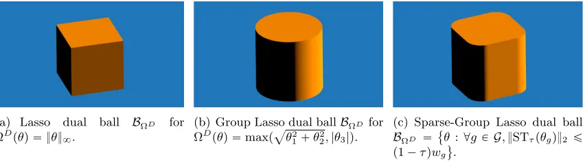
For the Sparse-Group Lasso, the geometry of the dual feasible set ∆X is more complex

(cf.Figure 3 for a comparison w.r.t. Lasso and Group Lasso). As a consequence, additional geometrical insights are needed to derive efficient safe rules, especially to compute the dual norm required by Equation (9) and the computation of the safe screening rules given in (7). We now introduce the -norm (denoted k¨k) as it has a connection with the

Sparse-Group Lasso norm Ωτ,w. The -norm was first proposed in Burdakov (1988) for other

purposes (see also Burdakov and Merkulov (2001)). For anyP r0,1sand anyxPRd,kxk

is defined as the unique nonnegative solution ν of the following equation (for “ 0, we definekxk_“0 :“kxk₈):

d ÿ

i“1

p|xi| ´ p1´qνq2` “ pνq

2_{. (17)}

Using soft-thresholding, this is equivalent to solve inνthe equationkST_p1´qνpxqk2“ν. Moreover, its dual norm is given by; see (Burdakov and Merkulov, 2001, Equation (42)):

kξkD “kξkD₂ ` p1´qkξkD<sub>8</sub> “kξk2` p1´qkξk1 . (18) This allows to express the Sparse-Group Lasso norm Ωτ,w using the dual -norm. We

Proposition 17 For all groups g in G, let us introduce g :“

p1´τqwg

τ` p1´τqwg

. Then, the

Sparse-Group Lasso norm satisfies the following properties: for any β and ξ in Rp,

Ωτ,wpβq “ ÿ

gPG

pτ` p1´τqwgq}βg}Dg and Ω

D

τ,wpξq “max_gPG

kξgk_g

τ ` p1´τqwg

.

B_ΩD

t,w “ ξPR

p _:@g

PG,kSTτpξgqk₂ ď p1´τqwg (

.

BΩτ,wpβq “ tzPRp :@gPG, zg PτBk¨k1pβgq ` p1´τqwgBk¨k2pβgqu.

Hence the dual feasible set is given by

∆X “ θPRn:@gPG,kSTτ `

X_gJθ˘k2 ď p1´τqwg (

“ θPRn:@gPG,kX_gJθk_g ďτ ` p1´τqwg (

.

Remark 18 Computing the dual norm of the Sparse-Group Lasso involves solving for each group g PG, a problem similar to the one given in (17) which has a quadratic complexity. To overcome this difficulty, an efficient algorithm relying on sorting techniques was proposed in (Ndiaye et al., 2016b, Prop. 5) to perform exact dual norm evaluation.

The Sparse-Group Lasso benefits from two levels of screening: the safe rules can detect both group-wise zeros and coordinate-wise zeros in the remaining groups: for any group g in G and any safe sphere Bpθ, rq, Equation (7) and the sub-differential of the Sparse-Group Lasso norm in Proposition 17 give (a detailed proof is given in (Ndiaye et al., 2016b, Appendix C))

Group level safe screening rule: max

θPBpθ,rq

kXJ g θkg τ ` p1´τqwg

ă1ñβˆ_gpλq“0.

Feature level safe screening rule: @jPg, max

θPBpθ,rq

|X_jJθ| ăτ ñβˆ_jpλq“0.

Noting that kSTτpxqk2 “ p1´τqwg ðñkxkg “τ` p1´τqwg, the above screening test on the group level can be rewritten as

max

θPBpθ,rq

ST_τpX_gJθq

2 ă p1´τqwg ñβˆ

pλq g “0.

The advantage of this formulation is that one can easily derive a “tight” upper-bound of the non-convex optimization problem in the left hand side of the preceding test. Indeed, we have STτpxq “x´ΠτB8pxq which brings us finally into a geometric problem easier to

solve. We recall from (Ndiaye et al., 2016b, Prop. 1) that for any centerθP∆X, any group

gPG and any jPg, we have the following upper-bound

max

θPBpθ,rq

|X_jJθ| ď |X_jJθ| `rkXjk₂,

max

θPBpθ,rq

ST_τpX_gJθq

2 ďTg:“

#

ST_τpX_gJθq

2`rkXgk2, if

X_gJθ

8 ąτ,

pX_gJθ

(a) Lasso dual ball BΩD for

ΩDpθq “ }θ}8.

(b) Group Lasso dual ballBΩD for

ΩDpθq “maxpaθ2

1`θ22,|θ3|q.

(c) Sparse-Group Lasso dual ball BΩD “ θ :@gP G,}STτpθgq}2 ď p1´τqwg

(

.

Figure 3: Lasso, Group Lasso and Sparse-Group Lasso dual unit balls: B_ΩD “ tθ: ΩDpθq ď 1u. For the illustration, the group structure is chosen such thatG“ tt1,2u,t3uu,

i.e.,g1“ t1,2u, g2 “ t3u,n“p“3,wg1 “wg2 “1 andτ “1{2.

Proposition 19 (Safe screening rule for the Sparse-Group Lasso)

Group level screening: @gPG, if Tg ă p1´τqwg, thenβˆgpλq “0.

Feature level screening: @gPG,@jPg, if |X_jJθ| `rkXjk₂ ăτ, thenβˆ_jpλq “0.

In the same spirit than Proposition 14, for any safe regionR,i.e.,a set containing ˆθpλq_, we define two levels of active sets, one for the group level and one for the feature level:

AgppRq:“ tgPG,max

θPR

ST_τpX_gJθq

2 ě p1´τqwgu,

AftpRq:“ ď

gPAgppRq

tjPg: max

θPR |X J

j θ| ěτu.

If one considers sequence of converging regions, then the next proposition (see (Ndiaye et al., 2016b, Prop. 3)) states that we can identify in finite time the optimal active sets defined as follows:

E_gp:“

!

gPG:

STτpX

J gθˆpλqq

2 “ p1´τqwg

)

, E_ft:“ ď

gPEgp !

jPg: |XJ

j θˆpλq| ěτ )

.

Proposition 20 Let pRkqkPN be a sequence of safe regions whose diameters converge to 0.

Then, lim

kÑ8

AgppRkq “Egp and lim

kÑ8

AftpRkq “Eft.

5.4 `1 Regularized Logistic Regression

Here, we consider the formulation given in (B¨uhlmann and van de Geer, 2011, Chapter 3) for the two-class logistic regression. In such a context, one observes for eachiP rnsa class label li P t1,2u. This information can be recast as yi “ 1tli“1u (where 1 is the indicator function), and it is then customary to minimize (3) where

Fpβq “

n ÿ

i“1

`

´yixJi β`log `

1`exp`xJ i β

˘˘˘

with fipzq “ ´yiz`logp1`exppzqq, and the penalty is simply the `1 norm: Ωpβq “ }β}1. Let us introduce Nh, the (binary) negative entropy function defined by:

Nhpxq “

#

xlogpxq ` p1´xqlogp1´xq, ifxP r0,1s ,

`8, otherwise . (20)

We use the convention 0 logp0q “0, and one can check thatf˚

i pziq “Nhpzi`yiqandγ “4.

Remark 21 We have privileged the formulation with the label y P t0,1un instead of y P t`1,´1unin order to be consistent with the multinomial cases below. One can simply switch from one formulation to the other thanks to the mapping yr“2y´1.

5.5 `1{`2 Multi-task Regression

The multi-task Lasso is a regression problem where the parameters form a matrix BPRpˆq. Denoting nthe number of observations for each task kP rqs, it is defined as

min BPRpˆq

1

2kY ´XBk 2

F `λ p ÿ

j“1

kBj,:k₂, (21)

where X P Rnˆp and Y P Rnˆq. Here we assume that the explanatory variables X are shared among the tasks however the Gap Safe rules would readily apply to the non-shared design formulation as in Lee et al. (2010) or in Liu et al. (2009) since the loss is still smooth (cf. Remark 7).

Introducing the vec operator that vectorizes a matrix by stacking its columns to form a column vector, and the Kronecker product b of two matrices, the multi-task Lasso can be rewritten as a special case of Group Lasso. In fact, we have n class of observations ci “ pi` pk´1qnqkPrqs of size q for each i P rns (the overall number of observations is

n1 _{“ nq) and p groups g}

j “ pj ` pk´ 1qpqkPrqs such that |gj| “ q for j P rps. The

design matrix ˜X “ Iq bX P Rn1ˆp1 “ Rnqˆpq is a q-block diagonal matrix defined as ˜

X“diagpX, . . . , Xq,y“vecpYq and β“vecpBq, we have:

min

βPRp1

1 2

n ÿ

i“1

y_ci´x˜J_i β

2 2`λ

p ÿ

j“1

β_gj

2, (22)

i.e., fipzq “ kyci ´zk 2

2{2. The advantage of this formulation is that it can be concisely written using the matrix forms ofy andβ, without the need to actually construct the large matrixX1_{. This is particularly appealing for the implementation.}

5.6 `1{`2 Multinomial Logistic Regression

We adapt the formulation given in (B¨uhlmann and van de Geer, 2011, Chapter 3) for the multinomial regression. In such a context, one observes for eachiP rnsa class labelli P rqs.

This information can be recast into a matrix Y PRnˆq filled by 0’s and 1’s: Yi,k “1tli“ku (where1is the indicator function). In the same spirit as for the multi-task Lasso, a matrix BPRpˆq is formed byq vectors encoding the hyperplanes for the linear classification. Thus the multinomial `1{`2 regularized regression reads:

min BPRpˆq

n ÿ

i“1

˜ _q ÿ

k“1

´Yi,kxJi B:,k`log ˜ _q

ÿ

k“1

exp`xJ i B:,k

˘ ¸¸

`λ

p ÿ

j“1

kBj,:k₂. (23)

Using a similar reformulation as in Section 5.5i.e.,definingci “ pi` pk´1qnqkPrqs for each

iP rnsandgj “ pj` pk´1qpqkPrqs for eachjP rps, the`1{`2 multinomial logistic regression can be cast into our framework as:

min

βPRp1

n ÿ

i“1 fi

` ˜

xJ_i β˘`λ

p ÿ

j“1

βgj

2, (24)

withfi:Rq ÑRsuch thatfipzq “ ´yJciz`log

` řq

k“1exppzkq

˘

. Note that generalizing (3) to functions fi:RqÑR does not bear difficulties, see Ndiaye et al. (2015).

Let us introduce NH, the negative entropy function defined by

NHpxq “

#_řq

i“1xilogpxiq, ifxPΣq“ txPR

q `:

řq

i“1xi“1u,

`8, otherwise. (25)

We use the convention 0 logp0q “0, and one can check thatf˚

i pzq “NHpz`Yiq andγ “1.

For multinomial logistic regression, Dλ implicitly encodes the additional constraintθP

domDλ “ tθ1PRn : @iP rns,´λθ1ci`yci PΣquwhere Σq is theq dimensional simplex, see Equation (25). By the dual scaling Equation (9), we have:

θ“Θ ˜

´GpXβq˜ λ

¸

“ R

maxpλ,ΩD_pXJ_Rqq, withR“y´RowNormpexppXβqq˜

where the function RowNorm consists in normalizing a (non-negative) matrix row-wise, such that each row sums to one. Thus for any iP rnsand α:“λ{maxpλ,ΩDpXJ_{Rqq P r0,1}

s,

´λθci`yci “ p1´αqyci`αRowNormpexppx˜

J i βqq

which is a convex combination of elements in Σq. Hence the dual scaling (9) preserves this

additional constraint.

6. Experiments

In this section we present results obtained with the Gap Safe rules on various data sets. Implementation9 has been done in Python and Cython (Behnel et al., 2011) for low level critical parts. A coordinate descent algorithm is used with a scaled dual gap stopping criterion i.e., we normalize the targeted accuracy (in the stopping criterion) in order to have a running time that is independent from the data scaling, i.e., Ð kyk2

2 for the regression cases andÐminpn1, n2q{nwhereni is the number of observations in the class

i, for the logistic cases.

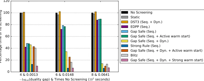
Note that in the Lasso case, to compare our method with the un-safe strong rules

by Tibshirani et al. (2012) and with the sequential screening rule such as theeddp+by Wang et al. (2012), we have added an approximated KKT post-processing step. We do this following Footnote 8, since they require the previous (exact) dual optimal solution which is not available in practice (Ndiaye et al., 2016b, Appendix B). The same limit holds true for theTLFreapproach of Wang and Ye (2014) addressing the Sparse-Group Lasso formulation, as well as for the method explored by Lee and Xing (2014) to handle overlapping groups and slores by Wang et al. (2014) for the binary logistic regression.

We have compared our method to various known safe screening rules (El Ghaoui et al., 2012; Xiang et al., 2011; Bonnefoy et al., 2014). For the Sparse-Group Lasso, such rules did not exist, so we have proposed natural extensions (Ndiaye et al., 2016b) thanks to exact computation of the dual norm in Proposition 17. For the Lasso estimator, we have also compared our implementation with theBlitz algorithm (Johnson and Guestrin, 2015) which combines Gap Safe screening rules, Prox-Newton coordinate descent and an active set strategy.

6.1 `1 Lasso Regression

Figure 4: Lasso on the Leukemia (dense data with n “ 72 observations and p “ 7129 features). fraction of the variables that are active. Each line corresponds to a fixed number of iterations for which the algorithm is run.

(a) Dense grid with 100 values ofλ.

(b) Coarse grid with 10 values ofλ.

Figure 5: Lasso on the Leukemia (dense data with n “ 72 observations and p “ 7129 features). Computation times needed to solve the Lasso regression path to desired accuracy for a grid ofλfrom λmaxtoλmax{103.

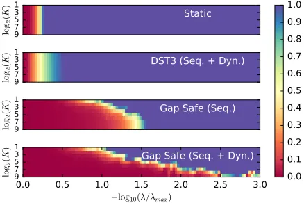
We have evaluated the computing time for the Gap Safe rules with and without active warm start, and compared with the static rule El Ghaoui et al. (2012) and the refined dynamic rule DST3 by Xiang et al. (2011), as well as Bonnefoy et al. (2015). We used the classic dense data set Leukemia, and the large sparse financial data set E2006-log1p available from LIBSVM10. We have normalized the column of X and standardized y to have zero mean and unit variance.

The experiments on Figure 4 focuses on the Leukemia data set. The screening per-formance for a fixed number of iterations, from 2 to 29, is investigated for each λ. It

demonstrates that increasing the number of iterations benefits to the dynamic screening rule. Also, the closer the estimate is from the global minimum, the better the screening. This is inline with the results in running time in the benchmark on Figure 5(a). Note that the dynamic Gap Safe rule is the only rule that significantly improves the running time of the Lasso.

(a) Dense grid with 100 values ofλ.

(b) Sparse grid with 10 values ofλ.

Figure 6: Lasso on financial data E2006-log1p (sparse data withn“16087 observations and p“1668737 features). Computation times needed to solve the Lasso regression path to desired accuracy for a grid ofλfrom λmax toλmax{20.

implementation combined with active or strong warm start. One advantage of our approach though, is the simplicity to insert it in any iterative algorithm as shown in Algorithm 1 and 2.

To demonstrate the limitations of the strong rules, we report in Figure 5(b) results with a coarse grid with only 10 values of λfrom λmax to λmax{103 such that 2λt ăλt´1. The strong rules become then useless since the screening test (14) selects all variables,

i.e.,ST Gpθˆpλt´1q_{, λ}

t, λt´1q “G. Overall, the greater the gap between grid points, the lower the benefits of (active) warm start.

In the experiment in Figure 6(b), we have stopped the grid at λmax{20 leading to a sparse solution with 1562 active variables. We obtain an important speed-up for both coarse and dense grids demonstrating the consistent efficiency of the active warm start strategy specially in a sparse regime.

Finally, with an extremely coarse grid, we therefore recommend the active warm start with the previous safe active set (which performance is only affected through the initializa-tion point) rather than the strong active set (cf.Figure 5(b)).

6.2 `1 Binary Logistic Regression

Results on the Leukemia data set for standard logistic regression are reported in Figure 7. We compare the dynamic strategy of Gap Safe to the sequential strategy. Results demon-strate the clear benefit of the dynamic rule in terms of high number of screened out variables. This is reflected in the graph of running times, which shows that dynamic Gap Safe rule with strong warm start can yield up to a 30ˆ speed-up compared to sequential rule and even more compared to an absence of screening (up to 50ˆspeed-up).

6.3 `1{`2 Multi-task Regression

To demonstrate the benefit of the Gap Safe screening rules for a multi-task Lasso problem we have considered neuroimaging data. Electroencephalography (EEG) and magnetoen-cephalography (MEG) are brain imaging modalities that allow to identify active brain re-gions. The problem to solve is a multi-task regression problem with squared loss where every task corresponds to a time instant. Using a multi-task Lasso one can constrain the recovered sources to be identical during a short time interval (Gramfort et al., 2012). This corresponds to a temporal stationary assumption. In this experiment we used a joint MEG/EEG data with 301 MEG and 59 EEG sensors leading ton“360. The number of possible sources is p “ 22,494 and the number of time instants is q “ 20. With a 1 kHz sampling rate it is equivalent to say that the sources stay the same for 20 ms.

(a) Fraction of the variables that are active. Each line corresponds to a fixed number of iterations for which the algorithm is run.

(b) Computation times needed to solve the logistic regression path to desired accuracy with 100 values ofλ

fromλmaxtoλmax{103.

Figure 7: `1 regularized binary logistic regression on the Leukemia (dense data withn“72 observations andp“7129 features). Sequential and full dynamic screening Gap Safe rules are compared.

6.4 Sparse-Group Lasso Regression

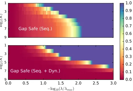
We consider the data set NCEP/NCAR Reanalysis 1 Kalnay et al. (1996) which contains monthly means of climate data measurements spread across the globe in a grid of 2.5˝

(a) Fraction of active variables as a function ofλand the number of iterations K. The Gap Safe strategy has a much longer range ofλ with (red) small active sets.

(b) Computation time to reach convergence using different screening strategies. We have run the algorithm with 100 values ofλfromλmax toλmax{103.

Figure 8: Experiments on MEG/EEG brain imaging data set (dense data with n “ 360 observations, p“22494 features andq “20 time instants).

(a) Proportion of active coordinate-wise variables as a function of parameterspλtqand the number of itera-tionsK.

(b) Proportion of active group variables as a function of parameterspλtqand the number of iterationsK.

(c) Time to reach convergence as a function of increasing prescribed accuracy, using various screening strategies and a logarithmic grid fromλmax toλmax{102.5.

Figure 9: Sparse-Group Lasso experiments on climate data NCEP/NCAR Reanalysis 1 (dense data with n “ 814 observations and p “ 73577 features) with τ “ 0.4 chosen by cross-validation.

We choose the parameterτ in the sett0,0.1, . . . ,0.9,1uby splitting in half the observa-tions, and run a training-test validation procedure. For each value ofτ, we require a duality gap of 10´8 _{on the training set and pick the best one in term of prediction accuracy on the} test set. Since the prediction error degrades increasingly forλďλmax{10´2.5_{, we fixδ“2.5.} We have fixed the weight wg “1 since all groups have the same size. The computational

7. Conclusion

We have proposed a unified presentation of the Gap Safe screening rules for accelerating algorithms solving supervised learning problems under sparsity constraints. The proposed approach applies to many popular estimators that boil down to convex optimization prob-lems where the data fitting term has a Lipschitz gradient and the regularization term is a separable sparsity enforcing function. We have shown that our methodology is more flexible than previously known safe rules as it conveniently unifies both regression and classification settings. The efficiency of the Gap Safe rules along with the newactive /strong warm start

strategies was demonstrated on multiple experiments using real high dimensional data set, suggesting that Gap Safe screening rules are always helpful to speed-up solvers targeting sparse regularization.

Acknowledgments

This work was supported by the ANR THALAMEEG ANR-14-NEUC-0002-01, the NIH R01 MH106174, by the ERC Starting Grant SLAB ERC-YStG-676943, by the Chair Ma-chine Learning for Big Data at T´el´ecom ParisTech and by the Orange/T´el´ecom ParisTech think tank Phi-TAB. We would like to thank the reviewers for their valuable comments which contributed to improve the quality of this paper.

References

A. Argyriou, T. Evgeniou, and M. Pontil. Multi-task feature learning. In NIPS, pages 41–48, 2006.

A. Argyriou, T. Evgeniou, and M. Pontil. Convex multi-task feature learning. Machine Learning, 73(3):243–272, 2008.

F. Bach, R. Jenatton, J. Mairal, and G. Obozinski. Convex optimization with sparsity-inducing norms. Foundations and Trends in Machine Learning, 4(1):1–106, 2012.

H. H. Bauschke and P. L. Combettes. Convex analysis and monotone operator theory in Hilbert spaces. Springer, New York, 2011.

A. Beck and M. Teboulle. A fast iterative shrinkage-thresholding algorithm for linear inverse problems. SIAM J. Imaging Sci., 2(1):183–202, 2009.

S. Behnel, R. Bradshaw, C. Citro, L. Dalcin, D.S. Seljebotn, and K. Smith. Cython: The best of both worlds. Computing in Science Engineering, 13(2):31 –39, 2011.

A. Bonnefoy, V. Emiya, L. Ralaivola, and R. Gribonval. A dynamic screening principle for the lasso. In EUSIPCO, 2014.

S. Boyd, N. Parikh, E. Chu, B. Peleato, and J. Eckstein. Distributed optimization and statistical learning via the alternating direction method of multipliers. Foundations and Trends in Machine Learning, 3(1):1–122, 2011.

P. B¨uhlmann and S. van de Geer. Statistics for high-dimensional data. Springer Series in Statistics. Springer, Heidelberg, 2011. Methods, theory and applications.

O. Burdakov. A new vector norm for nonlinear curve fitting and some other optimization problems. 33. Int. Wiss. Kolloq. Fortragsreihe ”Mathematische Optimierung — Theorie und Anwendungen”, pages 15–17, 1988.

O. Burdakov and B. Merkulov. On a new norm for data fitting and optimization problems.

Link¨oping University, Link¨oping, Sweden, Tech. Rep. LiTH-MAT, 2001.

A. Chambolle and T. Pock. A first-order primal-dual algorithm for convex problems with applications to imaging. J. Math. Imaging Vis., 40(1):120–145, 2011.

S. Chatterjee, K. Steinhaeuser, A. Banerjee, S. Chatterjee, and A. Ganguly. Sparse group lasso: Consistency and climate applications. InSIAM International Conference on Data Mining, pages 47–58, 2012.

B. Efron, T. Hastie, I. M. Johnstone, and R. Tibshirani. Least angle regression. Ann. Statist., 32(2):407–499, 2004. With discussion, and a rejoinder by the authors.

L. El Ghaoui, V. Viallon, and T. Rabbani. Safe feature elimination in sparse supervised learning. J. Pacific Optim., 8(4):667–698, 2012.

R.-E. Fan, K.-W. Chang, C.-J. Hsieh, X.-R. Wang, and C.-J. Lin. Liblinear: A library for large linear classification. J. Mach. Learn. Res., 9:1871–1874, 2008.

J. Fan and J. Lv. Sure independence screening for ultrahigh dimensional feature space. J. Roy. Statist. Soc. Ser. B, 70(5):849–911, 2008.

O. Fercoq, A. Gramfort, and J. Salmon. Mind the duality gap: safer rules for the lasso. In

ICML, pages 333–342, 2015.

J. Friedman, T. Hastie, H. H¨ofling, and R. Tibshirani. Pathwise coordinate optimization.

Ann. Appl. Stat., 1(2):302–332, 2007.

J. Friedman, T. Hastie, and R. Tibshirani. Regularization paths for generalized linear models via coordinate descent. Journal of statistical software, 33(1):1, 2010.

W. J. Fu. Penalized regressions: the bridge versus the lasso. J. Comput. Graph. Statist., 7 (3):397–416, 1998.

A. Gramfort, D. Strohmeier, J. Haueisen, M.S. Hmlinen, and M. Kowalski. Time-frequency mixed-norm estimates: Sparse M/EEG imaging with non-stationary source activations.

NeuroImage, 70(0):410 – 422, 2013.

J.-B. Hiriart-Urruty and C. Lemar´echal. Convex analysis and minimization algorithms. II, volume 306. Springer-Verlag, Berlin, 1993.

R. Jenatton, J. Mairal, G. Obozinski, and F. Bach. Proximal methods for hierarchical sparse coding. J. Mach. Learn. Res., 12:2297–2334, 2011.

T. B. Johnson and C. Guestrin. Blitz: A principled meta-algorithm for scaling sparse optimization. In ICML, pages 1171–1179, 2015.

T. B. Johnson and C. Guestrin. Unified methods for exploiting piecewise linear structure in convex optimization. InNIPS, pages 4754–4762, 2016.

E. Kalnay, M. Kanamitsu, R. Kistler, W. Collins, D. Deaven, L. Gandin, M. Iredell, S. Saha, G. White, J. Woollen, et al. The NCEP/NCAR 40-year reanalysis project. Bulletin of the American meteorological Society, 77(3):437–471, 1996.

K. Koh, S.-J. Kim, and S. Boyd. An interior-point method for large-scale l1-regularized logistic regression. J. Mach. Learn. Res., 8(8):1519–1555, 2007.

M. Kowalski, P. Weiss, A. Gramfort, and S. Anthoine. Accelerating ISTA with an active set strategy. In OPT 2011: 4th International Workshop on Optimization for Machine Learning, page 7, 2011.

S. Lee and E. P. Xing. Screening rules for overlapping group lasso. preprint arXiv:1410.6880v1, 2014.

S. Lee, J. Zhu, and E. P. Xing. Adaptive multi-task lasso: with application to eqtl detection. In NIPS, pages 1306–1314, 2010.

J. Liang, J. Fadili, and G. Peyr´e. Local linear convergence of forward–backward under partial smoothness. In NIPS, pages 1970–1978, 2014.

H. Liu, M. Palatucci, and J. Zhang. Blockwise coordinate descent procedures for the multi-task lasso, with applications to neural semantic basis discovery. InICML, pages 649–656, 2009.

E. Ndiaye, O. Fercoq, A. Gramfort, and J. Salmon. GAP safe screening rules for sparse multi-task and multi-class models. NIPS, pages 811–819, 2015.

E. Ndiaye, O. Fercoq, A. Gramfort, V. Leclere, and J. Salmon. Efficient smoothed concomi-tant Lasso estimation for high dimensional regression. Arxiv preprint arXiv:1606.02702, 2016a.