NUMERICAL SOLUTION OF AN INVERSE PROBLEM FOR THE LIOUVILLE EQUATION
F˙IKRET G ¨OLGELEYEN1, MUHAMMED HASDEM˙IR1,§
Abstract. We consider an inverse problem for the Liouville Equation. We present the solvability conditions and obtain numerical solution of the problem based on the finite difference approximation.
Keywords: Inverse problem, Liouville equation, finite difference method. AMS Subject Classification: 35R30, 65N21
1. Introduction
In this work, we consider the Liouville equation
Lu≡ ∂u
∂t +{H, u}=λ(x, v, t) (1)
in the domain Ω ={(x, v, t) :x∈D⊂Rn, v∈G⊂Rn, t∈(0, T)},where
{H, u}=
n X
i=1
∂H ∂vi
∂u ∂xi −
∂u ∂vi
∂H ∂xi
and the boundary∂Ω is sufficiently smooth.
In applications, u(x, v, t) is the density of distribution of the number of the particles in the phase space, H(x, v, t) is the Hamiltonian, λ(x, v, t) is a source function, x is the space coordinate vector,v and tdenote the velocity and time, respectively. The Liouville equation characterizes the continuity of the motion of a substance with phase volume conservation. It is used for quantitative and qualitative description of many physical, chemical, biological, social and other processes [3].
There have been many works on the direct problems for the Liouville equation, [See, e. g. 9]. As for the inverse problems, we refer to [1, 3], where the uniqueness of the solution was investigated. Numerical solution of some inverse problems for the stationary kinetic and transport equations were studied in [6-8]. To the best of our knowledge, there has been
1
Department of Mathematics, Zonguldak B¨ulent Ecevit University, 67100, Zonguldak, Turkey. e-mail: [email protected]; ORCID: https://orcid.org/0000-0002-8059-2194.
e-mail: [email protected]; ORCID: https://orcid.org/0000-0001-5901-3699. § Manuscript received: January 12, 2017; accepted: June 11, 2017.
TWMS Journal of Applied and Engineering Mathematics Vol.9, No.4 cI¸sık University, Department of Mathematics, 2019; all rights reserved.
no study devoted to numerical solution of such inverse problems for the non-stationary Liouville equation.
In this paper, we investigate the solvability conditions and numerical solution of the following inverse problem:
Problem 1. Determine the functions u(x, v, t) and λ(x, v, t) that satisfy equation (1) provided that the trace of the solutionu(x, v, t) on the boundary ∂Ω is known:
u|∂Ω=u0. (2)
The uniqueness of the solution of Problem 1 will be proved in the same way as in [1, p. 86], [3, p. 43].
Theorem 1. Let the Hamiltonian H(x, v, t)∈ C2 Ω
satisfy the conditions
n X
i,j=1 ∂2H ∂vi∂vj
ξiξj ≥α1|ξ|2, n X
i,j=1 ∂2H ∂xi∂xj
ξiξj ≤ −α2|ξ|2, (3)
for all (x, v, t) ∈ Ω , ξ ∈ Rn, where α1, α2 are positive numbers. We assume that the
function λ(x, v, t) satisfies the equation
b Lλ≡
n X
j=1 ∂2λ
∂vj∂xj = 0. (4)
Then Problem 1 has at most one solution (u, λ) such that u∈C2 Ω
, λ∈C2(Ω).
Proof. Let (u, λ) be a solution to Problem 1 such that u = 0 on ∂Ω and u ∈ C2 Ω,
λ∈C2(Ω). Since (4) holds for the function λ, we have
n X i=1 ∂u ∂vi ∂λ ∂xi = n X i=1 ∂ ∂vi u∂λ ∂xi . (5)
On the other hand, we can write
2 n X i=1 ∂u ∂vi ∂ ∂xi ∂u
∂t +{H, u} = n X i,j=1
∂2H ∂vi∂vj
∂u ∂xi
∂u ∂xj −
∂2H ∂xi∂xj ∂u ∂vi ∂u ∂vj + n X i=1 ∂ ∂t ∂u ∂vi ∂u ∂xi + ∂ ∂xi ∂u ∂vi ∂u
∂t +{H, u} − ∂ ∂vi ∂u ∂xi ∂u
∂t +{H, u} + n X i,j=1 ∂ ∂xj ∂H ∂vj ∂u ∂vi ∂u ∂xi − ∂ ∂vj ∂H ∂xj ∂u ∂vi ∂u ∂xi . (6)
Taking into account the geometry of the domain Ω and condition u= 0 on ∂Ω,from
(5)-(6),we get
n X i,j=1 Z Ω
∂2H ∂vi∂vj
∂u ∂xi
∂u ∂xj −
∂2H ∂xi∂xj ∂u ∂vi ∂u ∂vj
dΩ = 2
n X i=1 Z Ω ∂u ∂vi ∂λ
By condition (3), we have
α1 Z
Ω
|∇xu|2dΩ +α2 Z
Ω
|∇vu|2dΩ≤0. (8)
Since Ω is bounded and u = 0 on ∂Ω, inequality (8) implies u = 0 in Ω. Hence, by
equation (1), we have λ= 0 in Ω,which completes the proof of the theorem.
It is easy to check that condition (4) holds, for example, for any function λof the form
λ=λ1(x, t) +λ2(v, t),whereλ1 and λ2 are continuously differentiable functions.
As for the existence of the solution of Problem 1, we reduce the problem to the following one with homogeneous boundary data:
Problem 2. Determine (u, λ) from the relations
Lu = λ(x, v, t) +F(x, v, t), (9)
u|∂Ω = 0, Lλb = 0, (10)
provided that the boundary∂Ω is sufficiently smooth and the concordance conditions for the data are satisfied. In (9),F is a known function inH2(Ω).
Then the following theorem can be proven by the same method presented in [1] which is based on the Galerkin method and we will omit the proof here.
Theorem 2. Under the hypothesis of Theorem 1, there exists a solution (u, λ) of
Problem (2) in H1(Ω)×L2(Ω).
We note that the solvability of Problem 1 depends on the geometry of the domain Ω. Namely, it is necessary that Ω can be represented in the form of the direct product of the three domainsD,Gand (0, T).
Next, we give another problem where the geometry of the domain is not essential for the solvability.
Problem 3. Find a pair of functions (u(x, v), λ(x, v)) defined in D×G that satisfy the stationary form of equation (1) and the conditions
∇u|∂(D×G) =u0, ∇vλ|∂(D×G)=λ0, u(x0, v0) =u1, (11)
where (x0, v0) is a point in D×G.
Theorem 3. Under the hypothesis of Theorem 1, Problem 3 has at most one solution
(u, λ) such that u∈C2 D×G
, λ∈C2 D×G .
Proof. Suppose that (u, λ) is a solution to problem (3) such that u0=λ0 =u1 = 0. Using
relations (5)-(8) in the stationary case and by the fact that ∇vλ is given on the entire
boundary we obtain uxi =uvi = 0, i= 1,2, ..., n. Then equation (1) in the stationary case
implies λ= 0 in D×G. Since u(x0, v0) =u1 = 0, it follows that u≡0in D×G, which
completes the proof.
2. The Finite Difference Method
Now we concern with the construction of finite difference approximation for the following inverse problem:
Problem 4. Find (u, λ) from the relations
ut(x, v, t) +Hv(x, v, t)ux(x, v, t)−Hx(x, v, t)uv(x, v, t) =λ(x, v, t) +F(x, v, t), (12) u(x, v, t)|∂Ω= 0,
b Lλ= 0,
where Ω ={(x, v, t)| x∈(a, b)⊂R,v∈(c, d)⊂R, t∈(e, f)⊂R}.
By applying the operatorLbto both sides of equation (12), we get an auxiliary Dirichlet
boundary value problem for a third order partial differential equation:
utxv+uxvxHv−uvvxHx+uxxHvv−uvvHxx+uxvHvx−uvxHxv+uxHvvx−uvHxvx=F(x, v, t),
(13)
u|∂Ω= 0. (14)
By using the central finite difference formulas in (13)-(14), we obtain the following discrete version of the previous problem:
(−k2+k1) ˜uki−1,j−1+ (2k2−k3 +k5) ˜uki,j−1+ (−k1−k2) ˜uki+1,j−1
+ (−2k1+k4−k6) ˜uki−1,j+ (−2k4+ 2k3) ˜uki,j+ (2k1+k4+k6) ˜uki+1,j
+ (k1+k2) ˜uki−1,j+1+ (−2k2−k3−k5) ˜uki,j+1+ (k2−k1) ˜uki+1,j+1
+(k7)(˜uk+1i+1,j+1−u˜ik+1−1,j+1−u˜k+1i+1,j−1+ ˜uik+1−1,j−1−u˜i+1,j+1k−1 + ˜uki−−1,j+11
+˜uki+1,j−1 −1−u˜ki−−1,j1 −1) =fei,jk , i= 1, ..., I,j= 1, ..., J,k= 1, ..., K; (15)
˜
uk0,j= ˜ukI+1,j = ˜uki,0 = ˜uki,J+1 = ˜u0i,j = ˜uK+1i,j = 0,
i= 0,1, ..., I+ 1, j = 0,1, ..., J+ 1, k= 0,1, ..., K+ 1, (16)
whereI, J, Kare positive integers, ∆x= (b(I+1)−a), ∆v= (J+1)(d−c) and ∆t= (K+1)(f−e) are step sizes in the directions x, v, t, respectively. In (15), ˜uki,j is the finite difference approximation for the solution u(xi, vj, tk) = u(a+i∆x, c+j∆v, e+k∆t), hki,j is the finite difference
approximation for the function H(xi, vj, tk) = H(a+i∆x, c+j∆v, e+k∆t),fei,jk is the
approximation to the functionF(xi, vj, tk) =F(a+i∆x, c+j∆v, e+k∆t) and
k1 = h
k
i+1,j−hki−1,j
4 (∆x)2(∆v)2,k2 =
hki,j+1−hki,j−1
4 (∆x)2(∆v)2,
k3 =
hki+1,j−2hki,j+hki−1,j
(∆x)2(∆v)2 ,k4 =
hki,j+1−2hki,j+hki,j−1
(∆x)2(∆v)2 ,
k5 = h
k
i+1,j+1−2hki,j+1+hki−1,j+1−hki+1,j−1+ 2hki,j−1−hki−1,j−1
4 (∆x)2(∆v)2 ,
k6 =
hki+1,j+1−2hki+1,j+hki+1,j−1−hik−1,j+1+ 2hki−1,j−hki−1,j−1
4 (∆x)2(∆v)2 ,
k7 = 1
The approximate solution ˜uki,j of Problem 4 is obtained atI×J×K mesh points of Ω by solving the matrix equation
˜
Aue=Fe, (17)
where ˜A is a block tridiagonal banded matrix of the form
˜ A=
A(1) B(1) 0 · · · 0 C(2) A(2) B(2) . .. ...
0 C(3) . .. . .. 0
..
. . .. . .. . .. B(I−1)
0 . . . 0 C(I) A(I)
IJ K×IJ K
. (18)
In (18), the matricesA(i),B(i),C(i) are defined as follows
A(i) =
A(i,1)1 A(i,1)2 0 · · · 0
A(i,2)3 A(i,2)1 A(i,2)2 . .. ... 0 A(i,3)3 . .. . .. 0
..
. . .. . .. . .. A(i,J2 −1)
0 · · · 0 A(i,J)3 A(i,J)1
J K×J K
,i= 1,2, . . . , I;
B(i) =
B1(i,1) B2(i,1) 0 · · · 0
B3(i,2) B1(i,2) B2(i,2) . .. ... 0 B3(i,3) . .. . .. 0
..
. . .. . .. . .. B(i,J2 −1)
0 · · · 0 B3(i,J) B1(i,J)
J K×J K
, i= 1,2, ..., I −1;
C(i) =
C1(i,1) C2(i,1) 0 · · · 0
C3(i,2) C1(i,2) C2(i,2) . .. ... 0 C3(i,3) . .. . .. 0
..
. . .. . .. . .. C2(i,J−1)
0 · · · 0 C3(i,J) C1(i,J)
J K×J K
where
A(i,j)s =
fs(i, j) 0 · · · 0
0 fs(i, j) . .. ...
..
. . .. . .. 0
0 · · · 0 fs(i, j)
KxK ,
Bs(i,j) =
gs(i, j) (−1)
s(s−1)
(s−1)! a 0 · · · 0 (−1)(s+1)(s−1)
(s−1)! a gs(i, j) . .. . .. ...
0 . .. . .. . .. 0
..
. . .. . .. . .. (−(s1)−s(s1)!−1)a
0 · · · 0 (−1)(s(s−+1)1)!(s−1)a gs(i, j)
K×K ,
Cs(i,j) =
hs(i, j) (−1)
(s+1)(s−1)
(s−1)! a 0 · · · 0 (−1)s(s−1)
(s−1)! a hs(i, j) . .. . .. ...
0 . .. . .. . .. 0
..
. . .. . .. . .. (−1)(s(s+1)−1)!(s−1)a
0 · · · 0 (−(s1)−s(s1)!−1)a hs(i, j)
K×K ,
s = 1,2,3, j = 1,2, ..., J ,
and
f1(i, j) = −2k4+ 2k3, f2(i, j) =−2k2−k3−k5, f3(i, j) = 2k2−k3+k5, h1(i, j) = −2k1+k4−k6, h2(i, j) =k1+k2, h3(i, j) =k1−k2,
g1(i, j) = 2k1+k4+k6, g2(i, j) =−k1+k2, g3(i, j) =−k1−k2, a=k7.
In (17), Fe is a column matrix which consists of
e F =
h e
f1,11 ,fe1,1,2 , ...,fe1,1K,fe1,21 ,fe1,22 , ...,fe1,2K, ...,fe1,J1 ,fe1,J2 , ...,fe1,JK , ...,feI,JK iT
and ue is the solution vector:
e
u=u˜11,1,u˜21,1,, ...,u˜K1,1,u˜11,2,u˜21,2, ...,u˜K1,2, ...,u˜11,J,u˜1,J2 , ...,u˜K1,J, ...,u˜KI,JT. Finally, we obtainλnumerically from the difference equation
(˜uk+1i,j −u˜ki,j−1)
2∆t +k2
(˜uki+1,j−u˜ki−1,j)
2∆x −k1
(˜uki,j+1+ ˜uki,j−1)
2∆v −fe
k i,j = ˜λ
k i,j,
3. Numerical Experiments
In this section, we present numerical solution of three inverse problems of the form (9)-(10) by using the method developed in the previous section. The computations are performed using MATLAB R2014a program on a PC with Intel(R) Core(TM) i7-7700HQ CPU 2.80 GHz, 16 Gb memory RAM, running under Windows 10.
Example 1. Let us consider the problem of finding (u, λ) in Ω = (2,3)×(−1,1)×(0,1) from relations (9)-(10) provided that
H(x, v, t) = v2+ log(x),
F(x, v, t) = x3(v−2tv+ 2tv3−v3) +x2(6t2v4−9t2v2−6tv4−10tv3+ 9tv2
+10tv+ 5v3−5v) +x(−20t2v4+ 35t2v2+ 20tv4+ 12tv3 −35tv2−12tv−6v3+ 6v).
It is known that the exact solution of the inverse problem is
u(x, v, t) = xv(x−2)(x−3)(v2−1)(t2−t), λ(x, v, t) = t(t−1)(12v4−30v2+x2−5x+ 6).
In the following figures, we compare the exact solution with the calculated finite difference solution of the problem forI = 80, J = 200, K = 2,that is we consider 32000 mesh points.
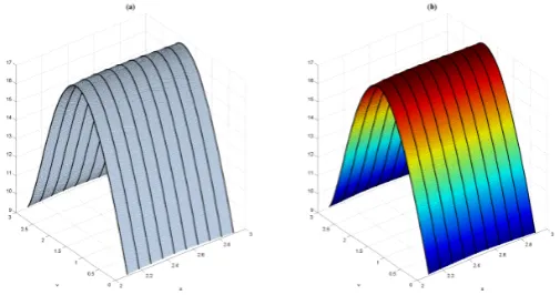
Figure 1. (a) Computed values and (b) Exact values of u for t=0.5.
Table 1. Errors in the computation for Example 1
I = 50, J = 100, I = 50, J = 200, I = 80, J = 200,
K = 2 K = 2 K = 2
Number of mesh points 10000 20000 32000
Elapsed time 90.42s 183.49 s 622.27 s
Figure 2. (a) Computed values and (b) Exact values ofλfor t=0.5.
0 0.5 1 1.5 2 2.5 3
x 104
0
0.5
1
1.5
2
2.5
3 x 10⁴
Figure 3. The structure of the matrix ˜A (32000×32000) in Example 1.
0 10 20 30 40 50 60 70 80
0 1 2 3 4 5 6 7 8 9x 10
−3 (a)
0 20 40 60 80 100 120 140 160 180 200
−8 −6 −4 −2 0 2 4 6 8x 10
−3 (b)
Computed Solution Exact Solution
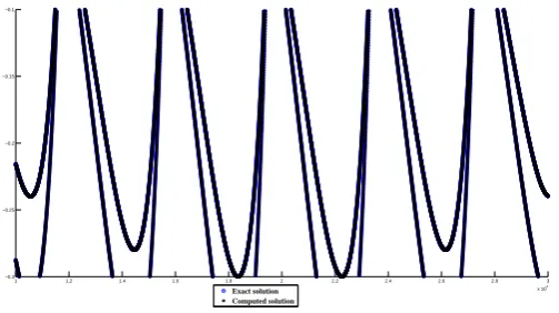
Figure 4. A comparison of computed and exact solutions for u:
(a) fixed v, t; (b) fixed x, t.
Example 2. Find a pair of functions (u, λ) defined in Ω = (2,3)×(0,3)×(0,1) that satisfies equation (9)-(10) with
H(x, v, t) = v
2
2 −x
2,
F(x, v, t) = x3(4tev−4t2ev−2tvev+ 2t2vev) +x2(v+ 3ev+ 20t2ev−2tv−26tev −vev+ 12tvev−10t2vev) +x(4tv−15ev−2t2v2−24t2ev−5v
The exact solution of the problem is
u(x, v, t) = (x−2)(x−3)(ev−1)(v−3)(t2−t),
λ(x, v, t) = x2(−2t2+ 2t)x3+ (10t2−4t−3) +x(−12t2−18t+ 15) + 36t+ 6v
+tv(5tv−5v−15t+ 3) +ev(v−3)(12t+ 5tv−5t2v−6)−18.
Figure 5. (a) Computed values and (b) Exact values of u for t=0.7.
Figure 6. (a) Computed values and (b) Exact values ofλfor t=0.7.
Table 2. Errors in the computation for Example 2
I = 4, J = 500, I = 10, J = 700, I = 10, J= 1300,
K = 4 K = 3 K= 3
Number of mesh points 8000 21000 39000
Elapsed time 39.11 s 214.51 s 1153.12 s
Maximum error for u 1.2796e-05 8.1005e-06 2.3519e-06
1 1.2 1.4 1.6 1.8 2 2.2 2.4 2.6 2.8 3 x 10⁴
−0.3 −0.25 −0.2 −0.15 −0.1
Exact solution Computed solution
Figure 7. A comparison of computed and exact solutions for u (all values).
Example 3. Find a pair of functions (u, λ) defined in Ω = (−3,3)×(0,1)×(1,3) that satisfies relation (9)-(10) with
H(x, v, t) = v
2
2 −x
2, F(x, v, t) = 1
t2
vx(3x−3vx)−tvx(−6v2+ 6v−12x2+ 108) +3vecos(πv2 +x))(x2−9)(v−1)
i
+1
t h
6xecos(πv2 +x))(−v3+v2−2vx2+ 18v+x2−9) +ecos(πv2 +x)sin(πv
2 +x)(x
2−9)(v2−v)(v+πx)(t2−4t+ 3)i
+vx(−8v2+vx+ 8v−16x2−x+ 144)−tvx(−2v2+ 2v−4x2+ 36)
−ecos(πv2 +x)x3(4tv−16v−2t+ 8) +x2(v2−v)
+x(18t+ 144v−36tv−2tv2+ 2tv3+ 8v2−8v3−72)−9v2+ 9v .
The exact solution of the problem is
u(x, v, t) = (t−3)(1
t −1)(e
cos(πv2 +x)−1)(x2−9)(v2−v), λ(x, v, t) = x3(8−6
t −2t) +x(18t+
54
t −72) + 9v+
1
t2(27v
2−27v)−9v2.
−3 −2 −1 0 1 2 3 0 0.2 0.4 0.6 0.8 1 −0.4 −0.2 0 0.2 0.4 0.6 0.8 1 1.2 1.4 1.6 x (a)
v −3 −2 −1 0 1 2 3
0 0.2 0.4 0.6 0.8 1 −0.4 −0.2 0 0.2 0.4 0.6 0.8 1 1.2 1.4 1.6 x v
Figure 8. (a) Computed values and (b) Exact values of u for t=2.
−3 −2 −1 0 1 2 3 0 0.1 0.2 0.3 0.4 0.5 0.6 0.7 0.8 0.9 1 −15 −10 −5 0 5 10 15 x (a) v −3 −2 −1 0 1 2 3 0 0.1 0.2 0.3 0.4 0.5 0.6 0.7 0.8 0.9 1 −15 −10 −5 0 5 10 15 x (b) v
Figure 9. (a) Computed values and (b) Exact values ofλfor t=2.
0 10 20 30 40 50 60 70 80 90 100
−0.05 0 0.05 0.1 0.15 0.2 0.25 0.3 (a)
0 10 20 30 40 50 60 70 80 90 100
−0.2 0 0.2 0.4 0.6 0.8 1 1.2 (b) exact solution computed solution
Figure 10. A comparison of computed and exact solutions for u:
Consequently, numerical experiments have demonstrated that the proposed method provides highly accurate numerical solutions for the source inverse problems for the Liou-ville equation. It is worth to note that the method used for proving the solvability of the inverse problem paves the way of solving the problem numerically. Namely, applying the operatorLb, our problem is reduced to a direct problem for u. Then the finite difference
approximation for the Dirichlet problem for a third order partial differential equation gives the result directly.
References
[1] Amirov, A. Kh., (2001), Integral Geometry and Inverse Problems for Kinetic Equations, VSP, Utrecht, The Netherlands.
[2] Anikonov, Yu. E. and Amirov, A. Kh., (1983), A uniqueness theorem for the solution of an inverse problem for the kinetic equation, Dokl. Akad. Nauk SSSR., 272 (6), pp. 1292-1293.
[3] Anikonov, Yu. E., (2001), Inverse Problems for Kinetic and other Evolution Equations, VSP, Utrecht, The Netherlands.
[4] Zhenglu, J., (2002), On the Liouville equation, Transport theory and statistical physics, 31 (3), pp. 267-272.
[5] Prilepko, A. I., Orlovsky, D. G. and Vasin, I. A., (2000), Methods for Solving Inverse Problems in Mathematical Physics, Marcel Dekker, Inc., New York.
[6] G¨olgeleyen, I., (2013), An inverse problem for a generalized transport equation in polar coordinates and numerical applications, Inverse problems, 29 (9), 095006.
[7] Amirov, A., Ustao˘glu, Z. and Heydarov, B., (2011), Solvability of a two dimensional coefficient inverse problem for transport equation and a numerical method, Transport theory and statistical physics, 40 (1), pp. 1-22.
[8] Amirov, A., G¨olgeleyen, F. and Rahmanova, A., (2009), An inverse problem for the general kinetic equation and a numerical method, CMES, 43 (2), pp. 131-147.
[9] Liboff, R. L., (2003), Kinetic Theory: Classical, Quantum, and Relativistic Descriptions, 3rd ed. Springer-Verlag, New York.
Fikret G ¨OLGELEYENreceived his BSc (2000) and MSc (2003) degrees in mathe-matics from Ondokuz Mayıs University and PhD degree (2010) in mathemathe-matics from Zonguldak B¨ulent Ecevit University (ZBEU). He conducted post-doctoral studies at the Graduate School of Mathematical Sciences, the University of Tokyo, in Japan. Since 2016, he has served as an associate professor in the Department of Mathematics at ZBEU in Turkey. His major research interests are inverse problems for differential equations, integral geometry problems and numerical analysis.