ISSN: 2008-6822 (electronic)
http://dx.doi.org/10.22075/ijnaa.2020.4264
A Method for Identifying Congestion Using
Non-Radial Models in Data Envelopment Analysis
A.R. Salehi, F. Hosseinzadeh Lotfi∗, M. Rostamy Malkhalifeh
Department of Mathematics, Science and Research Branch, Islamic Azad University, Tehran, Iran
(Communicated by Madjid Eshaghi Gordji)
Abstract
Data envelopment Analysis) DEA) is a nonparametric method that aims to use scientific methods in order to investigate the performance of Decision Making Unit (DMU). One of the interesting subjects in DEA is estimation of congestion of DMUs. Congestion problem has an important role in economy because the congestion mostly occurs in the input which is itself cost based, thus by eliminating congestion, the cost reduces as well. Therefore, detecting and reducing congestion both have many benefits. Many methods have been proposed to detect congestion in DEA. In this paper, we are going to present a new method to identify congestion based on the definition of congestion. The proposed method in this paper has the following advantages compare with other methods; Firstly, it is less complicated than other methods. Secondly, our method is able to identify the congestion and its degree correctly.thirdly the new model identifies the congestion of all units. Finally, the proposed method in this paper has non-radial movement.
Keywords: Data envelopment analysis, Efficiency, Inefficiency, Congestion, non-Radial models
1. Introduction
Data envelopment analysis (DEA) as a non-parametric technique has been widely used to measure the relative efficiency of a set of similar decision making units (DMUs) which was introduced in the year 1987 by Charnes and Cooper et al. (CCR model) [1]. Banker, Charnes and Cooper developed a variable returns to scale that was called BCC model in 1984 [2]. Congestion is often involved in the real practice which describes the case whereby the decrease of one (or some) inputs will cause the maximum possible increase of one (or some) outputs without worsening any other input or output [3].
∗Corresponding author
Email address: [email protected], [email protected], [email protected](A.R. Salehi, F. Hosseinzadeh Lotfi∗, M. Rostamy Malkhalifeh )
Proceeding in reverse, congestion occurs when the increases in one or more inputs can be associated with the decreases in one or more outputs without improving any other input or output. Fare et al. proposed a model to analysis congestion under the framework of DEA, which is widely recognized today [4]. FGL (Fare, Grosskopf and Lovell) approach uses a radial Farrell measure and is based on the assumption of strong and weak disposability of input [5]. It has been employed by a lot of studies into congestion. Cooper et al. proposed an alternative approach to measure congestion [6]. This approach is extended by Brockett et al. and was known as BCSW model [7]. BCSW model is a slack-based model which can recognize the congestion and identify sources of congestion and estimate congestion amounts [8]. Wei and Yan [9] and Tone and Sahoo [10] rebuilt the production possibility set (PPS) and the corresponding DEA model to determine the congestion effect of the DMUs. Jahanshahloo and Khodabakhshi develop a model based on relaxed combinations of inputs to make good input combinations and measure the amount of input congestion in textile industry of China [11]. Khodabakhshi provided a one-model approach of input congestion based on input relaxation model [12]. Sueyoshi and Sekitani proposed a modified approach which is able to measure congestion under the occurrence of multiple solution [13]. Noura et al. presented a new method for measuring congestion [14]. Kao utilize Wei-Tone model to measure the congestion effect of Taiwan forests [15]. Jahanshahloo et al. [16] and Khodabakhshi et al. [17] proposed some methods for computing the congestion in DEA models with production trade-offs and weight restrictions. There exist some papers which reviewed congestion papers, as that of Khodabakhshi et al. [18]. Hajihosseini et al. proposed a new approach for measuring the congestion in DMUs by using common weights based on comparison of inputs [19]. Some advantages and disadvantages of the aforementioned methods are mentioned below. FGL and BCSW Methods identify the congestion of the decision making unit but are not able to recognize the congestion type. In addition, FGL method may recognize the congestion of the decision making unit when there is no congestion, but may not recognize the congestion when it exists. In addition, Tone and Sahoo method is one of the best methods to identify the congestion in DEA. The first advantage of this method is to identify congestion condition (strong or weak) in a decision making unit. In addition, this method can accurately identify congestion for the DMUs. It should be noted there are a lot of problems in the presented methods to identify the congestion problems. For example, Tone and Sahoo method considers all inputs and outputs of DMU positively which is rarely happen in real world.This paper unfolds as follows. Section 2 provides some theoretical considerations. In section 3, we are going to present a new method to identify congestion based on the definition of congestion. Section 4 is devoted to a numerical example with real data and finally section 5 presents some concluding remarks.
2. Preliminaries
Suppose that there exist n decision making units,DM Uj,j = 1,· · · , n, and each DMU consumes
m inputs to produce s outputs. The i th input and r th output forDM Uj are denoted byxij andyrj,
respectively fori= 1,· · · , mand r= 1,· · · , s. We assume that all input and output values are non-negative, and at least one of each is non-zero. Let DM U o= (xo, yo) be the unit under assessment. The production Possibility Set (PPS) with variable returns to scale (VRS) defined Banker et al. is as follows [2]
Tv =
(
(x, y)|x≥ n
X
j=1
λjxj, y ≤ n
X
j=1
λjyj, n
X
j=1
λj = 1, λj ≥0, j = 1,· · · , n
)
The output-oriented BCC model for evaluating efficiency score ofDM Uo in its envelopment form is
as follows:
ψ∗ = maxρ+(
m
X
i=1
s−i +
s
X
r=1
s+i )
s.t. n
X
j=1
λjxij +s−i =xio i= 1,· · · , m
n
X
j=1
λjyrj −s+r =ρyro r = 1,· · · , s
n
X
j=1
λj = 1
λj ≥0 j = 1,· · · , n s−i ≥0 i= 1,· · · , m
s+r ≥0 r = 1,· · · , s (2.1)
Where is the non-Archimedean constant and variables s−i and s+
r are slacks. Now, we review three
main methods for estimation of congestion in the DEA framework.
2.1. FGL model
Fare, Grosskopf and Lovell proposed the model to estimate congestion using the following model (called FGL model) [5]:
β∗ = maxβ
s.t. n
X
j=1
λjxij =τ xio i= 1,· · ·, m
n
X
j=1
λjyrj ≥βyro r= 1,· · · , s
n
X
j=1
λj = 1
λj ≥0 j = 1,· · · , n
0≤τ ≤1 (2.2)
Suppose thatψ∗ andβ∗ represent the optimal objective values of model (2.1) and (2.2) respectively. It is clear that β∗ ≤ ψ∗, therefore βψ∗∗ ≤ 1. If
β∗
ψ∗ < 1 then DM Uo is congested, Otherwise, the
congestion will not be recognized using FGL model.
2.2. CTT model
Cooper et al. proposed an alternative DEA approach, called CTT, to estimate the congestion [6]. First, solve model (2.2) to evaluateDM Uo. Suppose that (ρ∗, s−∗, s+
∗
, λ∗) is the optimal solution for this model. Now, determine the benchmark of DM Uo on the strongly efficient frontier of Tv using
the following formulation:
c
xio =xio−s−i
∗
i= 1,· · · , m
c
yro =ρ∗yro+s+r
∗
It is clear that, ifDM Uo is on the strongly efficient frontier ofTv, then xb0 =x0,yb0 =y0.
Then, solve model (2.4) to determine the extent of the input congestion.
max
m
X
i=1
δi−
s.t. n
X
j=1
λjxij −δi−=xci0 i= 1,· · · , m
n
X
j=1
λjyrjyrc0 r= 1,· · · , s
n
X
j=1
λj = 1
λj ≥0 j = 1,· · · , n
0≤δi−≤s−i ∗ i= 1,· · · , m (2.4)
Thus, the extent of input congestion related to input xio can be described as:
sic =s−i ∗−δi−∗, i= 1,· · · , m. (2.5)
2.3. TS model
Tone and Sahoo defined PPS (called Pconvex) as follows [10]:
Pconvex =
(
(x, y)|x=
n
X
j=1
λjxj, y ≤ n
X
j=1
λjyj, n
X
j=1
λj = 1, λj ≥0, j = 1,· · · , n
)
(2.6)
Model (2.7) evaluates the efficiency score of DM Uo with respect to Pconvex:
Φ∗ = max Φ +(
m
X
i=1
s+r)
s.t. n
X
j=1
λjxij =xio i= 1,· · ·, m
n
X
j=1
λjyrj −s+r = Φyro r= 1,· · · , s
n
X
j=1
λj = 1
λj ≥0 j = 1,· · · , n
s+r ≥0 r= 1,· · ·, m (2.7)
The benchmark of DM Uo on the strongly efficient frontier of Pconvex is as follows:
c
xio =xio i= 1,· · · , m
c
yro = Φ∗yro+s+r
∗
Definition 2.1. The unit DM Uo = (xo, yo)∈Pconvex is strongly efficient with respect to Pconvex, if
Φ∗ = 0.
Definition 2.2. Suppose thatDM Uo = (xo, yo)∈Pconvex is strongly efficient with respect toPconvex.
This DMU is strongly congested if there exists an activity (xbo,ybo) ∈ Pconvex such that xbo = αxo
(0< α <1) and ybo ≥βyo(β >1).
Definition 2.3. The unit DM Uo= (xo, yo)∈Pconvex is (weakly) congested if it is strongly efficient
with respect to Pconvex. and there exists an activity in Pconvex that uses less resources in one or more inputs for making more products in one or more outputs.
Tone and Sahoo proposed the following method to determine the DMU’s situation of strong and weak congestion [10].
Step 1: Solve model (2.1). Therefore, we have:
(a) If ρ∗ = 1, s−∗ = 0, s+∗ = 0, then DM U
o = (xo, yo) is BCC-efficient and not congested.
(b) If ρ∗ = 1, s−∗ 6= 0, s+∗ = 0, then DM U
o = (xo, yo) is BCC-inefficient.
(c) If ρ∗ = 1, s+∗ 6= 0 orρ∗ >1, then DM U
o= (xo, yo) displays congestion. Go to step 2.
Step 2: solve model (2.9):
¯
u= maxu0
s.t. m
X
i=1
uryro = 1 i= 1,· · · , m
s
X
r=1
uryrj − m
X
i=1
vixij +uo ≤0 j = 1,· · · , n
s
X
r=1
uryro− m
X
i=1
vixio +uo = 0
ur ≥0 r = 1,· · · , s
vi f ree i= 1,· · · , m
uo f ree (2.9)
Suppose that ¯uis the optimal value of model (2.9), also assume that ¯ρ= 1 + ¯u. If ¯ρ <0 thenDM Uo
is strongly congested. If ¯ρ≥0 thenDM Uo is weakly congested.
3. Proposed Model
The definition of congestion requires to be discussed in both decrement and increment of inputs. In other words,DM Up has congestion, if and only if the following two conditions happen simultaneously
1- Decrement of the input leads to increment of the output for at least one component.
Suppose that there exist n decision-making units (DM Uj for j = 1,· · · , n) and each DMU uses
m inputs to produce s outputs. The ith input and rth output for DM Uj are specified by xij(i =
1,· · · , m) and yrj(r = 1,· · · , m), respectively. Banker et al. defined PPS (called ) with variable
return to scale (VRS) as follows [2]:
Tv =
(
(x, y)|x≥ n
X
j=1
λjxj, y ≤ n
X
j=1
λjyj, n
X
j=1
λj = 1, λj ≥0, j = 1,· · · , n
)
Because the principle of disposability of inputs is incompatible with the definition of congestion, therefore, we eliminate this principle from PPS to define congestion.
TN =
(
(x, y)|x=
n
X
j=1
λjxj, y ≤ n
X
j=1
λjyj, n
X
j=1
λj = 1, λj ≥0, j = 1,· · · , n
)
DM Up is congested, if and only if:
∀(¯x,y¯) (¯x,y¯)∈TN; ¯x≤6=xp =⇒y¯≥yp
∀(¯x,¯ y¯¯) (¯x,¯ y¯¯)∈TN; ¯x¯≥6=xp =⇒y¯≤yp
We consider whether there is a possibility of increasing the outputs in DM Up or not.
Z∗ = max1
s s
X
r=1
Φr
s.t. n
X
j=1
λjxij =tixip i= 1,· · · , m
n
X
j=1
λjyrj ≥Φryrp r= 1,· · · , s
n
X
j=1
λj = 1
λj ≥0 j = 1,· · · , n
Φr ≥1
The constraints ti ≥ 0, Φr ≥ 1 are caused that increasing in outputs is considered with decreasing
and increasing in inputs.
Z∗ = max 1
m m
X
i=1
si
s.t. n
X
j=1
λjxij =sixip i= 1,· · · , m
n
X
j=1
λjyrj ≥Φ∗ryrp r= 1,· · ·, s
n
X
j=1
λj = 1
λj ≥0 j = 1,· · · , n
si ≥0 (3.2)
Now, by solving model (3.2), we understand whether there exists a point (x, y) in TN such that at least one of the components of inputs and outputs of this unit be greater than the components of inputs and outputs ofDM Up.
Theorem 3.1. Suppose that (λ∗,Φ∗, t∗) is an optimal solution for model (3.1), (ˆλ,sˆ) is an optimal solution for model (2.2) and also Φ∗ ≥(1,· · · ,1), ˆs≤(1,· · · ,1) then DM Up is congested.
3.1. Recognizing the strong and weak congestion
Suppose that (λ∗,Φ∗, t∗) is an optimal solution for model (3.1), (ˆλ,ˆs) is an optimal solution for model (3.2) and also Φ∗ ≥(1,· · · ,1), ˆs≤(1,· · · ,1):
If Φ∗r ≥1 for all r= 1,· · ·, s and ˆs <1 then DM Up is strongly congested.
If Φ∗is not greater than 1 and ˆsis not less than 1 then we must recognizeDM Upis strongly congested or weakly congested. For this purpose, we solve the following models:
Z1∗ = max1
s.t. n
X
j=1
λjxij =tixip i= 1,· · · , m
n
X
j=1
λjyrj ≥Φryrp r = 1,· · · , s
n
X
j=1
λj = 1
λj ≥0 j = 1,· · ·, n
1
s s
X
r=1
Φr =Zo∗
Φr ≥1 +1
λj ≥0 j = 1,· · ·, n
Suppose that (λ∗, t∗,Φ∗, ∗1) is an optimal solution for model (3.3), therefore there exist the following cases:
If∗1 = 0, then all of the components of output of DM Up cannot be increased. Since Φ∗ ≥6=(1,· · · ,1)
in the optimal solution for model (3.1) and ˆs ≤ (1,· · ·,1) in the optimal solution for model (3.2) then, DM Up is weakly congested.
If∗1 = 0 then Φ∗ ≥1 +∗1 >1∀r.
That’s mean, all of the components of output can be increased. now, we solve model (3.4) to determine whether all of the components of input ofDM Up can be decreased or not.
Z3∗ = max2
s.t. n
X
j=1
λjxij =tixip i= 1,· · · , m
n
X
j=1
λjyrj ≥Φ∗ryrp r = 1,· · · , s
n
X
j=1
λj = 1
1
m s
X
r=1
ti =Z1∗
ti+2 ≤1
λj ≥0 j = 1,· · · , n
ti ≥0
2 ≥0 (3.4)
If (λ∗, t∗, ∗2) is an optimal solution for model (3.4), then there exist two the following cases: If∗2 = 0, then all of the components of input of DM Up cannot be decreased.
Since ˆs≤6=(1,· · · ,1) in the optimal solution for model (3.2) then, DM Up is weakly congested.
If∗2 >0, then t∗1 ≤1−∗2 <1∀i
And since, Φ∗r >1 for allr= 1,· · · , sthereforeDM Upis strongly congested and the size of congestion
in is equal toc1 = 1−t∗1. As regards, in the optimal solution of model (3.4),t∗i <1 for alli= 1,· · · , m,
therefore, Ci∗ > 1 for all i = 1,· · · , m. note that xp >0, because if xp = 0 then DM Up is efficient
with respect toTv, hence this unit is not congested. We consider a case that (λ∗,Φ∗, t∗) is the optimal
solution for model (3.1) in which Φ∗r = 1 for allr= 1,· · · , s. As regards, the components of output of units can’t be increased inTv then DM Up is not congested. Also in the optimal solution (λ∗,Φ∗, t∗)
for model (2.1) and in the optimal solution (ˆλ, s∗) for model (3.2), there exists I such that ˆsi < 1
then DM Up is not congested because, Φr ≥1 for allr= 1,· · ·, s cause that by increasing of the ith
component of input ofDM Up, all of the components of output of this unit are not decreased.
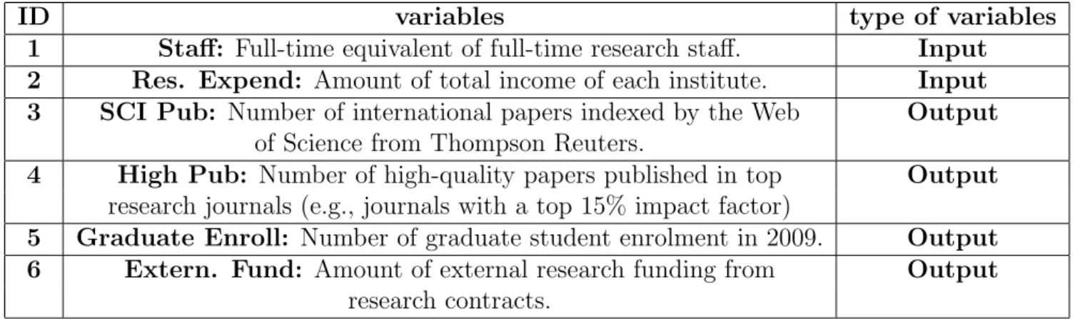
4. Numerical examples
Table 1: The inputs and outputs
ID variables type of variables
1 Staff: Full-time equivalent of full-time research staff. Input 2 Res. Expend: Amount of total income of each institute. Input 3 SCI Pub: Number of international papers indexed by the Web Output
of Science from Thompson Reuters.
4 High Pub: Number of high-quality papers published in top Output
research journals (e.g., journals with a top 15% impact factor)
5 Graduate Enroll: Number of graduate student enrolment in 2009. Output 6 Extern. Fund: Amount of external research funding from Output
research contracts.
The real data of two inputs and four outputs are shown in Table 2.
Table 2: Input-output data
DMU Staff Res. Expen SCI High Grad. E Exter. Fund. Φ∗o η∗
DM U1 252 117.945 436 133 184 31.558 1 0.2004
DM U2 37 29.431 243 127 43 15.3041 1 0.2004
DM U3 240 101.425 164 70 89 33.8365 1.1835 0.1485
DM U4 356 368.483 810 276 247 183.8434 1 0.4200
DM U5 310 195.862 200 55 111 12.9342 1.9684 0.3046
DM U6 201 188.829 104 49 33 60.7366 1.6499 0.3910
DM U7 157 131.301 113 49 45 72.5368 1.0437 0.3442
DM U8 236 77.439 8 1 44 23.7015 1 0
DM U9 805 396.905 371 118 89 216.9885 1 0.0878
DM U10 886 411.539 607 216 168 88.5561 1 0
DM U11 623 221.428 314 49 89 45.3597 1 0
DM U12 560 264.341 261 79 131 41.1156 1.4478 0.1715
DM U13 1344 900.509 627 168 346 645.4150 1 0
DM U14 508 344.312 971 518 335 205.4528 1 0.3134
DM U15 380 161.331 395 180 117 90.0373 1 0.1308
DM U16 132 83.972 229 138 62 32.6111 1.3371 0.2374
First, we solve model (3.2). This model determines that DM U3, DM U5, DM U8, DM U9, DM U10,
DM U11,DM U12,DM U15,DM U16are strongly congested. Then, we solve model (3.3) and recognize
that DM U1 and DM U4 are weakly congested. Finally, model (3.4) is solved and is determined that
DM U2 and DM U3 are weakly congested.
5. Conclusion
existence of congestion. Based on the first condition decrement of the input leads to increment of the output and in second condition increment of the input leads to decrement of the output. Models (3.1) and (3.2) were introduced based on the proposed definitions and model (3.3) and (3.4) should be solved in order to identify strong or weak congestion. According to numerical examples, for some DMUs, the decrement of the input was indicated, which led to increment of the output but increment of the input leads to increment of the output as well. Most of the congestion methods such as Cooper recognize this unit as congestion but based on the proposed definition in this paper, it doesn’t have congestion because the proposed method in this paper has this advantage to identify congestion with both increasing and decreasing input. In addition, our proposed method can determine that congestion has occurred in which unit of input and to what extent. Moreover, this method can determine which output unit and to what extent will increase if congestion is eliminated. The proposed models in this paper are non-radial and have the ability of identifying strong or weak congestion.
References
[1] A. Charnes, W. W. Cooper and E. Rhodes, Measuring the efficiency of decision-making units, Euro. J. Operational Research, 2(1978) 429-444.
[2] R.D. Banker, A. Charnes, W.W. Cooper, Some models for estimating technical and scale efficiencies in data envelopment analysis, Management Science, 30(1984) 1078-1092.
[3] W.W. Cooper, L.M. Seiford, J. Zhu, Handbook on data envelopment analysis, Kluwer Academic Publishers, Massachusetts, USA, (2004).
[4] R. F¨are, S. Grosskopf, Measuring congestion in production, Zeitschrilft f¨ur National¨okonomie, (1983) 257-271. [5] R. F¨are, S. Groskopf, C.A.K. Lovell, The Measuremen to Efficiency of Production, Kluwer Nijhoff Publishing,
Boston, (1985).
[6] W.W. Cooper, R.G. Thompson, R.M. Thrall, Introduction: extension and new developments in DEA, Annals of Operations Research 66(1996) 3-45.
[7] P.L. Brockett, W.W. Cooper, H.C. Shin, Y. Wang, Inefficiency and congestion in Chinese production before and after the 1978 economic reforms, Socio-Economic Planning Sciences, 32(1998) 1-20.
[8] W.W. Cooper, B.S. Gu, S.L. Li, Comparisons and evaluation of alternative approaches to the treatment of congestion in DEA, European Journal of Operational Research, 132(2001b) 62-67.
[9] Q.L. Wei, H. Yan, Congestion and returns to scale in data envelopment analysis, European Journal of Operational Research, 153(2004) 641-660.
treatment of congestion in DEA. European Journal of Operational Research 132, 62-67.
[10] K. Tone, B.K. Sahoo, Degree of scale economies and congestion: a unified DEA approach, European Journal of Operational Research, 158(2004) 755-772.
[11] G. R. Jahanshahloo, M. Khodabakhshi, Suitable combination of inputs for improving outputs in DEA with determining input congestion-Considering textile industry of China, Applied Mathematics and Computation, Vol. 151, No, 1(2004) 263-273.
[12] M. Khodabakhshi, A one-model approach based on relaxed combinations of inputs for evaluating input congestion in DEA, Journal of Computational and Applied Mathematics, 230(2009) 443-450.
[13] T. Sueyoshi, K. Sekitani, DEA congestion and returns to scale under an occurrence of multiple optimal projections, European Journal of Operational Research, 194 (2009) 592-607.
[14] A. A. Noura, F. Hosseinzadeh Lotfi, G. R. Jahanshahloo, S. Fanati Rashidi, B. R. Parker, A new method for measuring congestion in data envelopment analysis, Socio-Economic Planning Sciences, Vol. 44, No, 4(2010) 240-246.
[15] C. Kao, Congestion measurement and elimination under the framework of data envelopment analysis, 35 Inter-national Journal of Production Economics, 123(2010) 257-265.
[16] G. R. Jahanshahloo, M. Khodabakhshi, F. H. Lotfi, & R. M. Goudarzi, Computation of congestion in DEA models with productions trade-offs and weight restrictions, Applied Mathematical Sciences, Vol. 5, No, 14(2011) 663-676.
[18] M. Khodabakhshi, F. Hosseinzadeh Lotfi, & K. Aryavash, Review of input congestion estimating methods in DEA, Journal of applied mathematics, (2014).
[19] A. Hajihosseini, A. A. Noura, F. Hosseinzadeh Lotfi, A New Approach to Measuring Congestion in DEA with Common Weights. Indian Journal of Science and Technology, Vol. 8, No, 6(2015) 574.