Current sheet flapping in the near-Earth magnetotail: peculiarities of propagation and parallel currents

www.ann-geophys.net/34/739/2016/ doi:10.5194/angeo-34-739-2016

© Author(s) 2016. CC Attribution 3.0 License.

Current sheet flapping in the near-Earth magnetotail: peculiarities

of propagation and parallel currents

Egor V. Yushkov1,2, Anton V. Artemyev1,3, Anatoly A. Petrukovich1, and Rumi Nakamura4 1_{Space Research Institute, 84/32 Profsoyuznaya st., Moscow, 117997, Russia}

2_{Faculty of Physics, Lomonosov University, Leninskie Gory, Moscow, 119991, Russia}

3_{Department of Earth, Planetary, and Space Sciences and Institute of Geophysics and Planetary Physics, University of} California, Los Angeles, California, USA

4_{Space Research Institute (IWF), AAS, Graz, Austria}

Correspondence to:Egor V. Yushkov ([email protected])

Received: 9 March 2016 – Revised: 22 July 2016 – Accepted: 31 July 2016 – Published: 13 September 2016

Abstract. We consider series of tilted current sheet cross-ings, corresponding to flapping waves in the near-Earth magnetotail. We analyse Cluster observations from 2005 to 2009, when spacecraft visited the magnetotail neutral plane near X∈ [−17,−8], Y ∈ [−16,−2]RE (in the GSM sys-tem). Large separation of spacecraft allows us to estimate both local and global properties of flapping current sheets. We find significant variation in flapping wave direction of propagation between the middle tail and flanks. Th series of tilted current sheets represent the system of periodic, almost parallel currents with typical thickness of current filaments about L=0.4RE. The earthward gradients ofBz magnetic

field are reduced within this current system in comparison with the gradients in the quiet near-Earth magnetotail. The wavelength (i.e. a distance between two crossings of current sheets with the same orientations) of the flapping waves is larger than 2π Lfor most of observations. The velocity of flapping wave propagation is about ion bulk velocity and is significantly lower than the velocity of ion drift relative to electrons. We discuss possible drivers of flapping and esti-mate the amplitude of the total parallel current generated by flapping waves.

Keywords. Magnetospheric physics (magnetotail)

1 Introduction

The magnetotail current sheet (CS) is the key element of the Earth magnetosphere. In the tail, processes of magnetic en-ergy dissipation and charged particle acceleration initialise the storms and substorms (Baker et al., 1996; Angelopou-los et al., 2008). Dynamical properties of the magnetotail CS (e.g. the reconnection of stretched magnetic field lines, or CS bending and oscillations) have been thoroughly studied starting from the 1960s (see reviews by Lui, 2004; Schindler, 2006; Treumann and Baumjohann, 2013; Zelenyi and Arte-myev, 2013; and references therein). Flapping, how it is recognised now, is one of the most widespread types of CS activity (e.g. Zhang et al., 2002; Sergeev et al., 2004). However, other manifestations of CS dynamics (e.g. earth-ward plasma flows with dipolarisation fronts, formation of plasmoids) are also observed (Sharma et al., 2008; Baumjo-hann et al., 2007). One can distinguish two kinds of flap-ping motion: the vertical oscillations of the quasi-horizontal CSs (when the normalN to the CS plane is basically along thezaxis,|Nz|>0.8, and kink-like waves do not propagate)

and formation of tilted CSs (when the normal is significantly tilted,|Nz|<0.8, and kink-like waves can propagate along

the dusk–dawn direction) (see details of this classification in Rong et al., 2015). These tilted CSs propagate toward the magnetotail flanks and represent a nonlinear wave-like perturbations (i.e. the perturbation amplitude is comparable with a background magnetic field) of the main magnetic field component Bx (hereafter we use the GSM coordinate

to restore CS spatial profiles (e.g. Sergeev et al., 1998; Runov et al., 2012), investigate Hall electric field configuration in CSs (Wygant et al., 2005; Vasko et al., 2014), and test numer-ical models of CS instability (e.g. Karimabadi et al., 2003b; Sitnov et al., 2006; Zelenyi et al., 2009; Nakamura et al., 2009). The opportunity of four-spacecraft measurements of magnetic field provided by the Cluster mission was actively used to investigate details of the CS flapping (Runov et al., 2005a; Petrukovich et al., 2006, 2008; Rong et al., 2010).

The main statistics of the CS flapping at distances |X|> 15REwere collected during the first four years (2001–2004) of the Cluster mission (Runov et al., 2005a) and were sig-nificantly expanded by Geotail investigations in this region (Sergeev et al., 2006). Further, THEMIS (Runov et al., 2009) and Cluster/Double Star (Zhang et al., 2005) observations have confirmed the large-scale nature of the flapping mo-tion. Cluster spacecraft separation in 2001–2004 was varied between 300 and 4000 km. Thus, the Cluster tetrahedron re-solved the local (along the normal direction to the CS plane) gradients of magnetic field in flapping CS well but could not estimate variations in CS characteristics along the magneto-tail. These variations, being weak in the mid-tail, should be stronger in the near-Earth region (see case studies in Naka-mura et al., 2009; Panov et al., 2012a). The strong gradients of CS parameters along the x axis in this region are con-sidered as potential drivers for CS instabilities resulting in flapping motion (Erkaev et al., 2009; Pritchett and Coroniti, 2011; Panov et al., 2012b).

In the near-Earth magnetotail the tilted CSs were first stud-ied, using Double Star and Geotail single-spacecraft observa-tions (Zhang et al., 2005; Sergeev et al., 2006). However, the number of observations in this region was small and proper-ties of tilted CS flapping were not discussed. Thus, we use Cluster observations collected after 2004, when spacecraft crossed CSs at radial distances around∼15REand the dis-tances between spacecraft were large enough to study both the local (along the normal direction) CS configuration and the spatial gradient dBz/dx, which is usually much weaker

than the main cross-tail gradient dBx/dz (see, e.g., Rong

et al., 2014; Artemyev et al., 2015). The spacecraft trajec-tories allow us to study CS flapping motion in the midnight near-Earth magnetotail edge X∼ −15RE and at the deep dawn flanks with|X|,|Y| ∼(10−15) RE(throughout the pa-per we call both of these regions the near-Earth magnetotail).

2 Data set and analysis techniques

We selected 108 CS crossings from Cluster 2005–2009 ob-servations: 18 series with about 2–10 CS crossings in each and several individual crossings. The majority of statistics consists of observations in 2005 and 2006. In 2007 two of four Cluster spacecraft were very close to each other (in com-parison with distances to another pair of spacecraft). Thus, the Cluster tetrahedron was close to triangle with the corre-sponding problems of estimations of magnetic field gradients

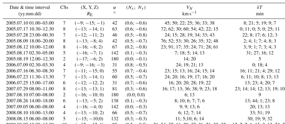
(Dunlop et al., 2002; Shen et al., 2012). In 2008 and 2009 we observe only few cases of flapping CSs (maybe due to evo-lution of spacecraft orbit). Table 1 shows all cases with the number of CS crossings and coordinates of the spacecraft tetrahedron centre for the first CS crossing.

We divide our statistics into two subsets: the first subset consists of individual CS crossings and the second subset consists of series of CS crossings. In all cases of our statis-tics the average angle betweenldirections of maximal mag-netic field variation (see description of the corresponding MVA method in Paschmann and Schwartz, 2000) obtained by four spacecraft is less than 10◦. Using the timing tech-nique (Runov et al., 2006) we determine the normal vec-torN, which is almost orthogonal to the l direction – the average angle is larger than 80◦. We do not use the MVA technique (see Paschmann and Schwartz, 2000, and refer-ences therein) to determine the normalndirection, because for many crossings the MVA technique provides two minor eigenvalues with close values. Due to the large distances be-tween spacecraft, we do not construct the local coordinate system (see, e.g., Runov et al., 2005b) by defining the direc-tion of current densityj=(c/4π )(∇ ×B)by the curlometer technique (Dunlop et al., 2002).

To apply the timing technique we determine the time de-lays between spacecraft observations of the same magnetic fieldBl. Due to the large distances, all four spacecraft often

do not cross the neutral plane for a selected CS crossing, so we approximateBl profiles by straight lines. The time

de-lays are defined as distances between these lines for a zero value ofBl. Then we calculate the velocity of the CS motion

along theNdirection,VNand the vectorN. The time delays

are also used to determine a period of CS oscillations,T, as an average time interval between the nearest crossings of CSs with the sameNvectors (within one series) and, correspond-ingly, the magnitude of the wavevectork=2π/(VNT ).

Nor-mal vectorN and anglesαbetween two successive normal vectorsNwithin one series characterise the CS tilt. Both ve-locityVNand time intervals between neighbouring CS

cross-ingsδT are presented in Table 1.

We use magnetic fieldBl=(B·l)to determine the

bound-ary magnetic field value B0 as a maximum|Bl| value for

a given CS crossing. We redefine Bz as a value of the z

component of magnetic fieldB with subtracted projection ofBl component to the zdirection. Large spacecraft

sepa-ration significantly averages current density peak and does not allow us to calculate current density amplitude. How-ever, the averaging does not change the current density di-rection, i.e. we can use curlometer data to estimate con-tributions of different current density components. Using this assumption we define the parallel current density as jk=(j×B)/|B|. However, we cannot use curlometer data to estimate small-scale gradients (e.g. current sheet thin-ness). Thus, we also determine the timing current density jtmg=(c/4π VN)∂Bl/∂t. This estimate of the current

be-Table 1.CS crossing characteristics: date and crossing time interval, number of CS crossings within a series, coordinates of the first CS crossing in GSM system (averaged from four spacecraft), angleαbetween two successive normal vectors (average value for entire series),

NxandNycomponents of the normal vector, velocityVNfor each crossing, and time delaysδT between CS crossings (averaged from four spacecraft).

Date & time interval CSs (X, Y, Z) α (Nx;Ny) VN δT

(yy.mm.dd) RE ◦ km s−1 min

2005.07.10 01.00–03.00 7 (−9;−15;−1) 42 (0.6;−0.6) 45; 50; 22; 25; 36; 33; 38 8; 21; 5; 19; 9; 7

2005.07.17 10.30–12.30 8 (−13;−14; 1) 63 (0.6;−0.6) 72; 62; 30; 60; 54; 42; 22; 15 0; 11; 0; 5; 0; 25; 11

2005.07.28 23.00–00.30 7 (−12;−11; 2) 46 (0.5;−0.8) 24; 15; 28; 19; 34; 33; 43 22; 8; 17; 6; 12; 3

2005.08.09 18.00–20.00 8 (−13;−8; 4) 42 (0.5;−0.7) 76; 52; 53; 30; 26; 35; 32; 48 2; 4; 1; 7; 4; 8; 3

2005.08.12 10.00–12.00 8 (−16;−8; 2) 67 (0.2;−0.8) 23; 91; 17; 35; 24; 71; 28; 61 3; 9; 1; 7; 3; 4; 3

2005.08.17 02.30–05.00 5 (−16;−7; 1) 142 (0.1;−0.3) 7; 18; 5; 14; 13 31; 27; 16; 12

2005.08.19 12.00–12.30 2 (−17;−6; 2) 180 (0.0;−0.1) 14; 20 5

2006.07.09 02.30–03.30 4 (−9;−16;−3) 31 (0.8;−0.5) 24; 19; 21; 13 0; 18; 4

2006.07.16 06.30–08.30 7 (−11;−15; 0) 55 (0.7;−0.4) 23; 15; 13; 16; 24; 15; 14 16; 11; 21; 4; 29; 12

2006.07.23 11.30–13.30 7 (−13;−14; 1) 60 (0.5;−0.7) 24; 20; 16; 19; 17; 16; 20 6; 11; 10; 8; 13; 13

2006.07.25 15.00–17.00 6 (−12;−12; 2) 31 (0.7;−0.6) 16; 20; 20; 28; 19; 22 13; 23; 4; 20; 7

2007.07.29 08.00–11.00 8 (−13;−13; 1) 81 (0.3;−0.6) 16; 17; 13; 36; 38; 9; 23; 18 23; 14; 14; 12; 13; 19; 10

2007.08.10 07.00–08.00 2 (−16;−10; 0) 180 (0.0; 0.0) 6; 13 9

2007.08.26 14.00–18.00 6 (−13;−5; 2) 138 (0.1;−0.3) 8; 10; 6; 7; 7; 6 13; 44; 1; 23; 8

2007.09.05 06.00–08.00 4 (−16;−4; 0) 142 (0.0;−0.3) 9; 9; 13; 6 20; 13; 13

2008.08.10 10.00–13.00 4 (−13;−10; 2) 66 (0.5;−0.7) 6; 12; 7; 14 33; 51; 19

2008.08.15 06.00–08.00 5 (−15;−10;0) 132 (0.3;−0.3) 11; 5;10; 6; 14 30; 19; 9; 32

2009.08.09 10.00–13.00 10 (−12;−12; 1) 98 (0.5;−0.5) 21; 54; 37; 16; 20; 37; 36; 21; 38; 32 12; 2; 7; 1; 15; 3; 13; 24; 23

cause the large distances between spacecraft strongly affect the accuracy of the curlometer technique and smooth mag-netic field gradients (see comparison betweenjcurlandjtmg for one CS crossing shown in Fig. 1c). Thus, for the estima-tion of the CS thicknessL we use the timing current den-sity amplitude:L=(c/4π )B0/jtmg(see Vasko et al., 2014). To study deformations of CS profiles we determine the stan-dard deviation dBzofBzmagnetic field in each CS crossing

interval. The CS configuration is verified using a standard deviationδBzof the magnetic fieldBzmeasured for

differ-ent CS crossings within each series: small δBz/hBzi value

shows that we deal with almost steady CS structures when onlyBl≈Bxvaries due to flapping motion.

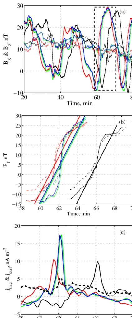
To demonstrate the application of all listed methods, we consider one event from our dataset shown in Fig. 1. This event includes series of seven tilted CSs crossed by four Cluster spacecraft at 28 July 2005 around(−12,−11,2) RE GSM. The average period of CSs oscillations is about 22 min. The maximum distance between spacecraft is∼1.7RE, and the minimum distance is ∼0.15RE. For each CS crossing from this series we determine the l direction (for all four spacecraft), two estimates of the current density jcurl and jtmg, and CS normal velocityVN. Deviation of theldirection

defined at different spacecraft does not exceed 1◦. To deter-mine time delays between spacecraft measurements of the same magnetic fieldBl, we approximate time profilesBl(t )

by straight lines using the least-squares method (see exam-ple in Fig. 1b). Knowing spacecraft positions and time de-lays, we calculate CS normal velocityVN≈28 km s−1.VN

is directed along the normal to CS, and the angle between the

normal direction andl direction varies between 83 and 96◦ for this event.

For each CS we calculate averaged values of theBz

mag-netic field excluding the component of Bz directed along

the l direction (for series shown in Fig. 1 we obtain Bz≈

14,16,12,11,9,8,7 nT). We also calculate the standard de-viation dBzofBzfor each CS crossing, e.g. dBz/Bz≈0.02

for CS crossings, shown in Fig. 1b. Knowing average Bz

values for all crossings from series, we calculate standard deviationδBz showing the difference between averagedBz

for one CS crossing and averagedBzfor all crossings from

series (δBz/hBzi ≈0.23 for series shown in Fig. 1). Using

average values ofBzmeasured by difference spacecraft, we

calculate gradients dBz/dx, dBz/dy, and dBz/dz.

Through-out the paper, we use the dBz/dx gradient (which for

se-lected series is equal to 0.4,0.7,0.6,0.2,0.1,0.6,0.5 nT/RE for seven CS crossings) and projection of the dBz/dr

gradi-ent onto thel direction, dBz/drl (which for selected series

is equal to 0.6,1.0,0.4,0.3,0.2,0.5,0.5 nT/REfor seven CS crossings). Similarly, we calculate gradients dφ/dx, dφ/dy of angleφbetween theldirection andx axis. These gradi-ents characterise the evolution of the orientation of the flap-ping wave front.

20 40 60 80 −10

0 10 20 30

Time, min B x

& B

z

, nT

(a)

58 60 62 64 66 68 70

−15 −10 −5 0 5 10 15 20 25 30

Time, min

B l

, nT

(b)

58 60 62 64 66 68 70

−5 0 5 10 15 20

Time, min

j tmg

& j

curl

, nA m

–2

(c)

Figure 1.Data from 28 July 2005 starting from 23:00 UTC.(a)Bx (dots) andBz (solid lines) fields in the series. The dash-bounded domain shows the example CS crossing. (b) Approximation of

Bl field used for calculation of time delays for the fourth cross-ing.(c)Amplitude of current density calculated by the curlome-ter method (dashed line) and the timing methodjtmg(solid lines for four spacecraft). Cluster spacecraft colours are black (1sc), red (2sc), green (3sc), and blue(4sc).

We also calculate the value ofBlcorresponding to the

max-imum of jtmg (in flapping CSs,jtmg can maximise at some

distance from Bl reversal, e.g. for the CS crossing shown

in Fig. 1b, Bl≈6.8 nT). To determine CS thickness

(spa-tial scale of current density variation) we use a ratio between Bl amplitude,B0, andjtmg magnitude. For selected series, B0varies from crossing to crossing within the range of 23– 32 nT, whereas CS thicknessL∈ [1.5,5.1]×1000 km. Using the period of CS oscillations, dT, we define a wavenumber k≈2π/(VNdT )and calculate thekLfactor.

3 Statistics of CS parameters

Coordinates of all CS crossings in(X, Y )and(Y, Z)planes are demonstrated in Fig. 2a and b. Straight lines show the directions of the CS motion,N. In agreement with previous observations (Sergeev et al., 2004; Runov et al., 2005a), al-most all observed CSs propagate toward the magnetosphere flank. Thus, we can interpret theBx magnetic field

oscilla-tions as the manifestation of wave-like disturbance propagat-ing away from the central (midnight) region of the magneto-tail. The periodic change of thezcomponent of theNvector within one series of CS crossings supports this conclusion. Figure 2 shows that all waves are observed forY <0: long series of CS crossings are mostly observed for|Y|>10RE, and small series including up to four crossings are usually observed closer to the midnight. Moreover, from Fig. 2b we see that, in region (|Y|<10RE), almost vertical oscillations of the quasi-horizontal CSs are observed (theN direction is along the±zdirection), whereas at the flank the main com-ponent of theNvector is along they direction (i.e. we deal with the dawnward propagation of titled CSs; see Table 1). Figure 2 shows that the direction of theN vector varies sig-nificantly from middle tailY ∼0 to flank|Y|>10RE. This effect was mentioned for mid-tail (Runov et al., 2005a), but in the near-Earth region it looks much more clear.

We use collected statistics of normal vectorsNto study the configuration of tilted CSs. For the mid-tail (X∼ −18RE) Petrukovich et al. (2006) showed that, in tilted CSs, the cur-rent density amplitude increases with the inclination of the neutral plane (i.e. with the growth of|Ny| component and

the decrease in the |Nz| component). These observations

were interpreted as an evidence of slip-like CS deforma-tions (i.e the kink of the neutral plane CS withoutBz

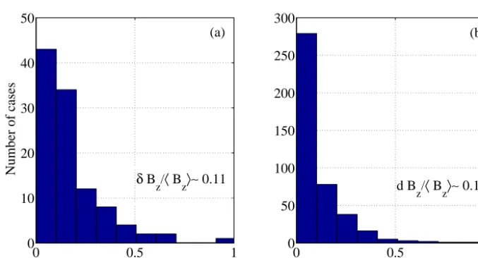
vari-ation; Petrukovich et al., 2008; Rong et al., 2010). Indeed, the histogram in Fig. 3a demonstrates that the standard de-viation of theBz magnetic field component from the value hBzi(averaged in each series) is quite small – the averaged

value δBz/hBzi is about 0.17 (both δBz and average hBzi

are calculated for series of CS crossings). The series with substantialBzvariations generally include cases with

mono-tonically decreasing ofBz(i.e. the CS stretching events; see,

e.g., Petrukovich et al., 2007). The example of significantBz

variation is shown in Fig. 1, where a gradual decrease inBz

is noticeable. Therefore, we can conclude that there are no periodic (or quasi-periodic) perturbations ofBzwith

re-−16 −14 −12 −10 −8 −18

−16 −14 −12 −10 −8 −6 −4 −2

X, R E

Y, R

E

−15 −10 −5

−3 −2 −1 0 1 2 3 4 5 6

Y, R E

Z, R

E

(a) (b)

Figure 2.CS crossings (dots) and vectorsNin the(X, Y )plane(a)and in the(Y, Z)plane(b).

0 0.5 1

0 50 100 150 200 250 300

dB z/〈 Bz〉

0 0.5 1

0 10 20 30 40 50

δ B z/〈 Bz〉

Number of cases

(a) (b)

d B

z/〈 Bz〉∼ 0.17

δ B

z/〈 Bz〉∼ 0.11

Figure 3. (a)Ratio of standard deviationδBz and magnetic field amplitudehBziaveraged for different CS crossings within each series. (b)Ratio of standard deviation dBzand magnetic field amplitudehBziaveraged for each CS crossing.

gion, and that field lines in the CS centre are slipping with the dominantBzcomponent (Petrukovich et al., 2008; Rong

et al., 2011). These observations provide the important limi-tation for models of flapping waves (see Discussion).

Several theoretical models predict the substantial varia-tions in Bz withx in oscillating CSs (Erkaev et al., 2009;

Pritchett and Coroniti, 2010; Sitnov et al., 2014). The large distances between Cluster spacecraft allow us to investigate the homogeneity of the flapping wave within spatial scale around 104km (i.e. size of the Cluster tetrahedron). Figure 3b shows the distribution of the standard deviation dBz

calcu-lated for individual CS crossings by four spacecraft. This de-viation is as small as 0.1Bz. Therefore, we could not find any

significant variations inBzwithin the spatial scale of

space-craft separation. Moreover, for all observed CSs, thel direc-tions calculated for different spacecraft coincide. Thus, we

can conclude that flapping CSs in the near-Earth magneto-tail are more or less uniform in the(X, Y )plane within the spatial scales about 1–2RE. This result confirms the previ-ously reported THEMIS observations of large-scale flapping motion (Runov et al., 2009; Kubyshkina et al., 2014).

In the near-Earth magnetotail we expect to observe rel-atively strong gradients of Bz along the x axis (Kan and

Baumjohann, 1990; Wang et al., 2009; Artemyev et al., 2013). The gradients∂Bz/∂x,∂Bz/∂y and∂Bz/∂rl, where

rl=(r·l), of magnetic field in the current sheet centre is

calculated for each crossing by means of the curlometer tech-nique (Runov et al., 2005a) and presented in Fig. 4. The dis-tribution of∂Bz/∂xis centred around zero but has a

signif-icant tail with∂Bz/∂x >0. These positive strong gradients

−2 0 2 0

5 10 15 20 25 30 35 40

Number of cases

dB

z/dx = 0.30 nT/RE

−2 0 2

0 5 10 15 20 25 30 35 40

dB

z/dy = −0.12 nT/RE

−2 0 2

0 5 10 15 20 25 30 35 40

dB

z/drl = 0.05 nT/RE

Figure 4.The gradients∂Bz/∂x,∂Bz/∂yand∂Bz/∂rlof magnetic fieldBzin the CS centre for each CS crossing.

0 0.5 1 1.5

0 10 20 30 40 50 60 70 80

L, R E

Number of cases

0 0.5 1 1.5 2 2.5 0

10 20 30 40 50 60 70 80

(L ⋅ k)

(a) (b)

L ∼ 0.44 R_{E (L⋅ k) ∼ 0.64}

Figure 5. (a)The statistics of CS thicknessL, calculated byB0andjtmgfor each CS crossing.(b)The distributionkLfor CS thicknessL and wavevectork.

−300 −20 −10 0 10 20 30 20

40 60 80 100

B l nT

Number of cases

B l∼ 3.7 nT

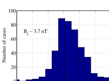
Figure 6.The position of the current density peakjtmgrelativeBl magnetic field.

1 nT/ REis attributed to observations at the flank magneto-tail, where previous statistics show average values∂Bz/∂x∼

0.5 nT/ RE(Wang et al., 2009; Rong et al., 2014). However, the majority of observed CSs correspond to|∂Bz/∂rl|<0.2

with an average value of about∼0. Thus, statistics of flap-ping CSs represent the subset of CSs with reduced∂Bz/∂x

gradients.

Estimates of∂Bz/∂xallow us to compare the typical scale

Lx∼Bz(∂Bz/∂x)−1and the CS thicknessL(scale of

mag-netic field variation along the normal direction). Figure 5a shows that the average current sheet thickness L is about 0.4RE. The average value of∂Bz/∂rl gradient derived from

statistics shown in Fig. 4 is smaller than 0.1 nT/ RE. Thus, the typical longitudinal sizeLx of tilted CS can be roughly

estimated as∼50RE forBz∼5 nT. The CS configuration

we deal with the 2-D structure, while`1 corresponds to a quasi-1-D CS (Burkhart and Chen, 1993). In our case the estimates give`1 due toLx/L∼125.

Figure 6 demonstrates the distribution of Bl value

corre-sponding to the peak value of the current densityjtmg. One can see that the average value of the distribution is positive (Bl∼4 nT) – i.e. there is a regular shift of the position of

the current density peak relative to theBlreversal. This shift

can be explained by the model of the kink CS deformation (Petrukovich et al., 2008; Rong et al., 2010). Moreover, we can suggest that the dominance of positive values ofBlshift

is due to the dominance of CS crossings with positivez co-ordinates (i.e. the CS neutral plane is shifted relative to the geometrical neutral plane z=0). Due to the peculiarity of the Cluster orbit we do not have enough statistics to check whether this asymmetry changes the sign forz <0.

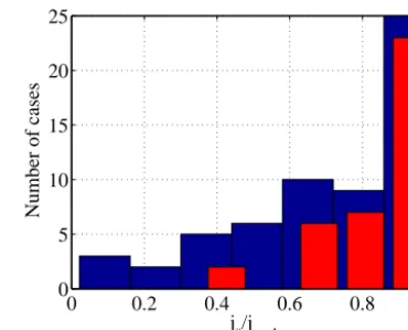
The distribution of ratio of parallel and total current den-sities is presented in Fig. 7. For almost all CSsjkrepresents more than 60 % of the total current density. Moreover, cases with smalljkcorrespond to the vertical flapping motion with N parallel tozaxis, whereas in CSs with smallNz

compo-nent (i.e. CSs corresponding to flapping wave propagation toward the flank), almost all of the current is parallel to the magnetic fieldB. This is the typical situation for tilted CSs, where the current density flows along the zaxis andBz is

large enough (Petrukovich et al., 2003; Shen et al., 2008; Vasko et al., 2014). Strong jz current density results from

deformation of the CS neutral plane (i.e.jz∼∂Bx/∂y)due

to flapping motion (see models in Petrukovich et al., 2008; Rong et al., 2010). Moreover, to verify this result, we check that, for most of the CSs from our statistics, the value of m×j/|j|is about 1 forj derived from the curlometer and mderived from MVA and timing methods. Thus, in the near-Earth magnetotail the CS flapping motion generates of strong parallel currents.

Using the estimates of the CS flapping velocity VN and

periodT (about∼20 min) we compare wavelength 2π/ k=

VNT and CS thicknessL. Figure 5b shows thatkLis

gen-erally less than 1 (the averaged value is 0.64). Thus, we deal with long wavelength perturbations of CSs. The deformation of CS neutral plane likely does not change the interval CS structure on small scales, but redistributes current density be-tween horizontal and vertical directions.

The directions of front prorogationN are calculated from four-spacecraft data and have rather low accuracy. On the other hand, the directions of the l vectors are estimated quite well at each spacecraft and the large distances between spacecraft allow us to investigate the configuration of the front. Figure 8a and b show that the averaged gradient (cal-culated for each CS crossings) dφ/dxof the angleφbetween theldirection andxaxis is negative (−2.5◦/ RE) and dφ/dy is positive (2.0◦/ RE) (φ=0 whenlis parallel toxaxis and φ= −90◦whenlis parallel toy axis). This means that the front configuration is most likely linear and azimuthally ro-tating than spherical and propagating from midnight, because

0 0.2 0.4 0.6 0.8 1

0 5 10 15 20 25

Number of cases

j ||/jcurl

Figure 7.Ratio of currents jk parallel to the magnetic field and total currentsj(blue for all cases and red only for tilted CSs with

|Nz|<0.7).

in the last case dφ/dy should be negative. Taking into ac-count that the gradient∂Bz/∂rlis close to zero (see Fig. 4),

we can suggest that (1) a midnight source of flapping waves runs them along constant levels of theBzfield and (2) wave

propagating results in the front rotation without a reconfigu-ration.

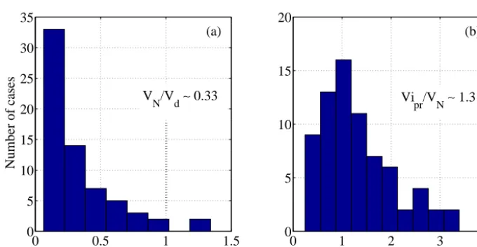
Figure 9 helps to compare a CS flapping velocityVN and

typical plasma velocities, such as the drift velocity Vd= jtmg/(ene)and the projection of the ion velocityVionto the N direction,V ipr. The electron densityne and ion velocity Viare taken from the PEACE experiment onboard C2 (John-stone et al., 1997) and the CIS/HIA experiment onboard C1 (Rème et al., 2001) respectively. Figure 9a demonstrates that the CS flapping velocityVN is usually less than the drift

ve-locity amplitudeVd=jtmg/(ene)(the average value of their ratio is 0.33 and more than 95 % of cases less then 1). Fig-ure 9b shows that the ratio of projection of ion bulk velocity andVN is about 1 (about 90 % of all cases are distributed

within the interval[0.5;2]).

4 Discussion

−20 −10 0 10 20 0

5 10 15 20 25 30 35 40 45

dφ /dx, degree/R E

Number of cases

−20 −10 0 10 20 0

5 10 15 20 25 30 35 40 45

dφ /dy, degree/R E dφ/dx ∼ −2.5 dφ/dy ∼ 2.0

(a) (b)

Figure 8.Gradients of the angle between thelvector andxaxis:(a)dφ/dxand(b)dφ/dy.

0 0.5 1 1.5

0 5 10 15 20 25 30 35

V N/Vd

Number of cases

0 1 2 3 4

0 5 10 15 20

Vi pr/VN V

N/Vd∼ 0.33 Vipr/VN∼ 1.3

(a) (b)

Figure 9. (a)Ratio of flapping wave velocity and drift velocityVN/Vd.(b)Ratio of ion bulk velocity and flapping wave velocityV ipr/VN.

The connection between magnetotail dynamics and iono-sphere processes involves the generation of parallel current systems in the near-Earth region. Statistics of current den-sity distribution in flapping CSs (see Fig. 7) show that strong deformation of the CS neutral plane can generate field-aligned currents. Amplitude of jz current density in tilted

CSs reaches 5–15 nA m−2(see Fig. 1 and statistics in Runov et al., 2005a; Vasko et al., 2014) and exceed dawn–dusk cur-rent density in quite magnetotail. If we assume thatjz

repre-sents a new current system generated likely by field-aligned electron flows in tilted CSs, we can estimate corresponding amplitudes of parallel currents in flapping magnetotail. Flap-ping perturbations seem to have large scales in the (X, Y ) equatorial plane due to the efficient decrease in gradients ∂/∂x in flapping CSs (see Fig. 4). The typical scale of a CS along thex axis is larger than (or comparable with)∼2RE (at such distances the tilted CSs are observed simultaneously

by Cluster spacecraft in events collected in our statistics), while the scale along theyaxis for a tilted CS isL∼0.3RE. Thus, a single tilted CS corresponds to the total current about

∼2RE×0.3RE×10 nA m−2∼0.2 MA.

pertur-bation of the Bz component δBz/Bz should be comparable

with a relative perturbation of theBxcomponent. However,

we observe a very weak perturbation ofδBz/Bz∼0.2 and

a very strong perturbation of δBx/Bx∼1. Moreover, we

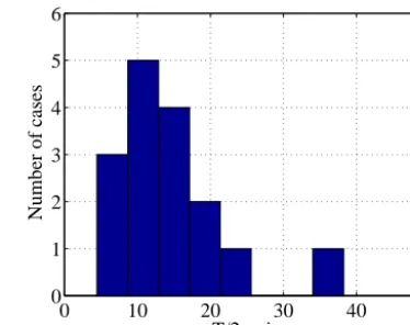
can compare periods of flapping waves (see Fig. 10) with predictions of double-gradient instability (Erkaev et al., 2009): dTmodel≈2π/p(dBz/dx)(dBx/dz)/(4π mpne)≈ 2π(4π L2mpne/B02)1/2/

√

2`, where mp is the proton mass and `=2(B0/L)/(dBz/dx). For dBz/dx≈dBz/dr≈

0.05nT/RE (see Fig. 4) and L≈0.44RE (see Fig. 5), we obtain dTmodel≈3–10 min for average values ofB0≈30 nT and ne≈0.3 cm−3. Observational periods of flapping motion vary between 9 and 25 min (see Fig. 10) – i.e. only fast oscillating CSs can be described by this model, whereas slowly oscillating CSs are too thin and intense to be described by the model of double-gradient instability (to have dTmodel≈25 min we need L≈1.5RE). Balloon-ing/interchange instability can also run flapping-like waves with flankward propagation (Pritchett and Coroniti, 2010). However, this instability requires the significant gradient dBz/dx <0, whereas we find only a weak (a value around

zero) or positive gradient dBz/dx (see Fig. 4). Kink modes

of CS instability (Daughton, 1999; Karimabadi et al., 2003a; Zelenyi et al., 2009) predict the flapping wave velocity about a drift velocity (due to strong diamagnetic drifts in the initial CS). Configuration of titled CSs assumes that current carrying particles (i.e. relative velocity of ions and electrons along the current density direction) flow almost along magnetic field lines, whereas CS flapping motion is in the transverse direction. Thus, we can estimate both ion drift velocityVi(i.e. velocity along the dawn–dusk direction) and current carrier velocity Vd (i.e. ratio of the current density and plasma density amplitudes). Our observations show that flapping velocity is comparable with observed ion bulk velocityViand is much smaller thanVd(see Fig. 9). There-fore, kink modes of CS instability can explain flapping wave propagation but cannot describe the dominance of parallel currents with largeVd(most models of kink waves consider zero or vanishing Bz; e.g. Daughton, 1999; Karimabadi

et al., 2003a; Zelenyi et al., 2009). Finally, we come to the puzzling conclusion that all three different instabilities (double-gradient, ballooning/interchange, and kink) meet difficulties in the explanation of observed flapping waves. Thus, further investigation of CS motion with significant parallel currents should be performed for explanation of observed flapping waves. Such parallel currents are likely carried by electrons (as was suggested and tested by Runov et al., 2006; Vasko et al., 2014).

5 Conclusions

In this paper we present the statistics of flapping CSs ob-served in the near-Earth magnetotail. The main our findings can be summarised as follows:

0 10 20 30 40 50

0 1 2 3 4 5 6

T/2, min

Number of cases

Figure 10.Distribution of flapping wave periods for our dataset.

– Despite the relatively strong gradients ∂Bz/∂x in the

background CS in the near-Earth tail (Kan and Baumjo-hann, 1990; Artemyev et al., 2013; Rong et al., 2014), this gradient is significantly reduced in flapping CSs (∼0.2 nT/RE). Moreover, a weak-gradient dBz/dx

found in the flapping near-Earth magnetotail questions models of double-gradient and ballooning/interchange instabilities as main candidates for excitation of flap-ping waves (Erkaev et al., 2009; Pritchett and Coroniti, 2010).

– The velocity of flapping wave probation is close to ion bulk velocityViand is much smaller than current carrier velocityVd=jtmg/(ene). The wavelength of flapping motion is larger than CS thickness (kL <1). These ob-servations point to a drift nature of flapping waves. – Flapping waves in the near-Earth magnetotail

gen-erate strong parallel currents with an amplitude of about∼0.2 MA and have a transverse spatial-scaleL smaller than the wavelength (i.e. typical distance be-tween neighbourhood structures) and typical periods of about∼20 min.

6 Data availability

All data were downloaded from Cluster Science Archive (ESA, 2016) (http://www.cosmos.esa.int/web/csa).

Acknowledgements. We are thankful to I. Y. Vasko for useful discussions. The authors would like to acknowledge the Cluster Active Archive, Cluster Science Archive, and Cluster instrument teams, in particular the FGM team for excellent data. The work of E. V. Yushkov, A. V. Artemyev, and A. A. Petrukovich was sup-ported by the Russian Foundation for Basic Research (project no. 14-05-91000). The work of R. Nakamura was supported by the Aus-trian Science Fund (FWF I2016-N20).

References

Angelopoulos, V., McFadden, J. P., Larson, D., Carlson, C. W., Mende, S. B., Frey, H., Phan, T., Sibeck, D. G., Glassmeier, K., Auster, U., Donovan, E., Mann, I. R., Rae, I. J., Rus-sell, C. T., Runov, A., Zhou, X., and Kepko, L.: Tail Recon-nection Triggering Substorm Onset, Science, 321, 931–935, doi:10.1126/science.1160495, 2008.

Artemyev, A. V., Petrukovich, A. A., Nakamura, R., and Zelenyi, L. M.: Profiles of electron temperature andBzalong Earth’s mag-netotail, Ann. Geophys., 31, 1109–1114, doi:10.5194/angeo-31-1109-2013, 2013.

Artemyev, A. V., Petrukovich, A. A., Nakamura, R., and Zelenyi, L. M.: Two-dimensional configuration of the magnetotail current sheet: THEMIS observations, Geophys. Res. Lett., 42, 3662– 3667, doi:10.1002/2015GL063994, 2015.

Baker, D. N., Pulkkinen, T. I., Angelopoulos, V., Baumjohann, W., and McPherron, R. L.: Neutral line model of substorms: Past results and present view, J. Geophys. Res., 101, 12975–13010, doi:10.1029/95JA03753, 1996.

Baumjohann, W., Roux, A., Le Contel, O., Nakamura, R., Birn, J., Hoshino, M., Lui, A. T. Y., Owen, C. J., Sauvaud, J.-A., Vaivads, A., Fontaine, D., and Runov, A.: Dynamics of thin current sheets: Cluster observations, Ann. Geophys., 25, 1365– 1389, doi:10.5194/angeo-25-1365-2007, 2007.

Burkhart, G. R. and Chen, J.: Particle motion in x-dependent Harris-like magnetotail models, J. Geophys. Res., 98, 89–97, doi:10.1029/92JA01528, 1993.

Daughton, W.: The unstable eigenmodes of a neutral sheet, Phys. Plasmas, 6, 1329–1343, doi:10.1063/1.873374, 1999.

Dunlop, M. W., Balogh, A., Glassmeier, K.-H., and Robert, P.: Four-point Cluster application of magnetic field anal-ysis tools: The Curlometer, J. Geophys. Res., 107, 1384, doi:10.1029/2001JA005088, 2002.

Erkaev, N. V., Semenov, V. S., Kubyshkin, I. V., Kubyshkina, M. V., and Biernat, H. K.: MHD model of the flapping motions in the magnetotail current sheet, J. Geophys. Res., 114, A03206, doi:10.1029/2008JA013728, 2009.

ESA: Cluster Science Archive, available at: http://www.cosmos.esa. int/web/csa, last access: 7 September 2016.

Jacobs, J. A., Kato, Y., Matsushita, S., and Troitskaya, V. A.: Clas-sification of Geomagnetic Micropulsations, J. Geophys. Res., 69, 180–181, doi:10.1029/JZ069i001p00180, 1964.

Johnstone, A. D., Alsop, C., Burge, S., Carter, P. J., Coates, A. J., Coker, A. J., Fazakerley, A. N., Grande, M., Gowen, R. A., Gur-giolo, C., Hancock, B. K., Narheim, B., Preece, A., Sheather, P. H., Winningham, J. D., and Woodliffe, R. D.: Peace: a Plasma Electron and Current Experiment, Space Sci. Rev., 79, 351–398, doi:10.1023/A:1004938001388, 1997.

Kan, J. R. and Baumjohann, W.: Isotropized magnetic-moment equation of state for the central plasma sheet, Geophys. Res. Lett., 17, 271–274, doi:10.1029/GL017i003p00271, 1990. Karimabadi, H., Daughton, W., Pritchett, P. L., and Krauss-Varban,

D.: Ion-ion kink instability in the magnetotail: 1. Linear theory, J. Geophys. Res., 108, 1400, doi:10.1029/2003JA010026, 2003a. Karimabadi, H., Pritchett, P. L., Daughton, W., and Krauss-Varban, D.: Ion-ion kink instability in the magnetotail: 2. Three-dimensional full particle and hybrid simulations and comparison with observations, J. Geophys. Res., 108, 1401, doi:10.1029/2003JA010109, 2003b.

Korovinskiy, D. B., Divin, A. V., Erkaev, N. V., Semenov, V. S., Artemyev, A. V., Ivanova, V. V., Ivanov, I. B., Lapenta, G., Markidis, S., and Biernat, H. K.: The double-gradient magnetic instability: Stabilizing effect of the guide field, Phys. Plasmas, 22, 012904, doi:10.1063/1.4905706, 2015.

Kubyshkina, D. I., Sormakov, D. A., Sergeev, V. A., Semenov, V. S., Erkaev, N. V., Kubyshkin, I. V., Ganushkina, N. Y., and Dubyagin, S. V.: How to distinguish between kink and sausage modes in flapping oscillations?, J. Geophys. Res., 119, 3002– 3015, doi:10.1002/2013JA019477, 2014.

Lui, A. T. Y.: Potential Plasma Instabilities For Sub-storm Expansion Onsets, Space Sci. Rev., 113, 127–206, doi:10.1023/B:SPAC.0000042942.00362.4e, 2004.

McPherron, R. L.: Magnetic Pulsations: Their Sources and Relation to Solar Wind and Geomagnetic Activity, Surv. Geophys., 26, 545–592, doi:10.1007/s10712-005-1758-7, 2005.

Nakamura, R., Retinò, A., Baumjohann, W., Volwerk, M., Erkaev, N., Klecker, B., Lucek, E. A., Dandouras, I., André, M., and Khotyaintsev, Y.: Evolution of dipolarization in the near-Earth current sheet induced by near-Earthward rapid flux transport, Ann. Geophys., 27, 1743–1754, doi:10.5194/angeo-27-1743-2009, 2009.

Panov, E. V., Nakamura, R., Baumjohann, W., Kubyshkina, M. G., Artemyev, A. V., Sergeev, V. A., Petrukovich, A. A., Angelopou-los, V., Glassmeier, K.-H., McFadden, J. P., and Larson, D.: Ki-netic ballooning/interchange instability in a bent plasma sheet, J. Geophys. Res., 117, A06228, doi:10.1029/2011JA017496, 2012a.

Panov, E. V., Sergeev, V. A., Pritchett, P. L., Coroniti, F. V., Naka-mura, R., Baumjohann, W., Angelopoulos, V., Auster, H. U., and McFadden, J. P.: Observations of kinetic ballooning/interchange instability signatures in the magnetotail, Geophys. Res. Lett., 39, L08110, doi:10.1029/2012GL051668, 2012b.

Panov, E. V., Baumjohann, W., Nakamura, R., Kubyshkina, M. V., Glassmeier, K.-H., Angelopoulos, V., Petrukovich, A. A., and Sergeev, V. A.: Period and damping factor of Pi2 pulsations dur-ing oscillatory flow brakdur-ing in the magnetotail, J. Geophys. Res., 119, 4512–4520, doi:10.1002/2013JA019633, 2014.

Paschmann, G. and Schwartz, S. J.: ISSI Book on Analysis Methods for Multi-Spacecraft Data, vol. 449 of ESA Special Publication, 2000.

Petrukovich, A. A., Baumjohann, W., Nakamura, R., Balogh, A., Mukai, T., Glassmeier, K.-H., Reme, H., and Klecker, B.: Plasma sheet structure during strongly northward IMF, J. Geophys. Res., 108, 1258, doi:10.1029/2002JA009738, 2003.

Petrukovich, A. A., Zhang, T. l., Baumjohann, W., Nakamura, R., Runov, A., Balogh, A., and Carr, C.: Oscillatory magnetic flux tube slippage in the plasma sheet, Ann. Geophys., 24, 1695– 1704, doi:10.5194/angeo-24-1695-2006, 2006.

Petrukovich, A. A., Baumjohann, W., Nakamura, R., Runov, A., Balogh, A., and Rème, H.: Thinning and stretch-ing of the plasma sheet, J. Geophys. Res., 112, 10213, doi:10.1029/2007JA012349, 2007.

Petrukovich, A. A., Baumjohann, W., Nakamura, R., and Runov, A.: Formation of current density profile in tilted current sheets, Ann. Geophys., 26, 3669–3676, doi:10.5194/angeo-26-3669-2008, 2008.

growth phase magnetotail stretching intervals, J. Geophys. Res., 118, 5720–5730, doi:10.1002/jgra.50550, 2013.

Pritchett, P. L. and Coroniti, F. V.: A kinetic ballooning/interchange instability in the magnetotail, J. Geophys. Res., 115, A06301, doi:10.1029/2009JA014752, 2010.

Pritchett, P. L. and Coroniti, F. V.: Plasma sheet disruption by interchange-generated flow intrusions, Geophys. Res. Lett., 381, L10102, doi:10.1029/2011GL047527, 2011.

Rème, H., Aoustin, C., Bosqued, J. M., Dandouras, I., Lavraud, B., Sauvaud, J. A., Barthe, A., Bouyssou, J., Camus, Th., Coeur-Joly, O., Cros, A., Cuvilo, J., Ducay, F., Garbarowitz, Y., Medale, J. L., Penou, E., Perrier, H., Romefort, D., Rouzaud, J., Vallat, C., Alcaydé, D., Jacquey, C., Mazelle, C., d’Uston, C., Möbius, E., Kistler, L. M., Crocker, K., Granoff, M., Mouikis, C., Popecki, M., Vosbury, M., Klecker, B., Hovestadt, D., Kucharek, H., Kuenneth, E., Paschmann, G., Scholer, M., Sckopke, N., Seiden-schwang, E., Carlson, C. W., Curtis, D. W., Ingraham, C., Lin, R. P., McFadden, J. P., Parks, G. K., Phan, T., Formisano, V., Amata, E., Bavassano-Cattaneo, M. B., Baldetti, P., Bruno, R., Chion-chio, G., Di Lellis, A., Marcucci, M. F., Pallocchia, G., Korth, A., Daly, P. W., Graeve, B., Rosenbauer, H., Vasyliunas, V., Mc-Carthy, M., Wilber, M., Eliasson, L., Lundin, R., Olsen, S., Shel-ley, E. G., Fuselier, S., Ghielmetti, A. G., Lennartsson, W., Es-coubet, C. P., Balsiger, H., Friedel, R., Cao, J.-B., Kovrazhkin, R. A., Papamastorakis, I., Pellat, R., Scudder, J., and Sonnerup, B.: First multispacecraft ion measurements in and near the Earth’s magnetosphere with the identical Cluster ion spectrometry (CIS) experiment, Ann. Geophys., 19, 1303–1354, doi:10.5194/angeo-19-1303-2001, 2001.

Rong, Z. J., Shen, C., Petrukovich, A. A., Wan, W. X., and Liu, Z. X.: The analytic properties of the flapping current sheets in the earth magnetotail, Planet. Space Sci., 58, 1215–1229, doi:10.1016/j.pss.2010.04.016, 2010.

Rong, Z. J., Wan, W. X., Shen, C., Li, X., Dunlop, M. W., Petrukovich, A. A., Zhang, T. L., and Lucek, E.: Sta-tistical survey on the magnetic structure in magnetotail current sheets, J. Geophys. Res.-Space, 116, A09218, doi:10.1029/2011JA016489, 2011.

Rong, Z. J., Wan, W. X., Shen, C., Petrukovich, A. A., Baumjohann, W., Dunlop, M. W., and Zhang, Y. C.: Radial distribution of mag-netic field in earth magnetotail current sheet, Planet. Space Sci., 103, 273–285, doi:10.1016/j.pss.2014.07.014, 2014.

Rong, Z. J., Barabash, S., Stenberg, G., Futaana, Y., Zhang, T., Wan, W. X., Wei, Y., and Wang, X. D.: Technique for diagnosing the flapping motion of magnetotail current sheets based on single-point magnetic field analysis, J. Geophys. Res., 120, 3462–3474, doi:10.1002/2014JA020973, 2015.

Runov, A., Sergeev, V. A., Baumjohann, W., Nakamura, R., Ap-atenkov, S., Asano, Y., Volwerk, M., Vörös, Z., Zhang, T. L., Petrukovich, A., Balogh, A., Sauvaud, J.-A., Klecker, B., and Rème, H.: Electric current and magnetic field geometry in flap-ping magnetotail current sheets, Ann. Geophys., 23, 1391–1403, doi:10.5194/angeo-23-1391-2005, 2005a.

Runov, A., Sergeev, V. A., Nakamura, R., Baumjohann, W., Zhang, T. L., Asano, Y., Volwerk, M., Vörös, Z., Balogh, A., and Rème, H.: Reconstruction of the magnetotail current sheet structure us-ing multi-point Cluster measurements, Planet. Space Sci., 53, 237–243, doi:10.1016/j.pss.2004.09.049, 2005b.

Runov, A., Sergeev, V. A., Nakamura, R., Baumjohann, W., Ap-atenkov, S., Asano, Y., Takada, T., Volwerk, M., Vörös, Z., Zhang, T. L., Sauvaud, J.-A., Rème, H., and Balogh, A.: Local structure of the magnetotail current sheet: 2001 Cluster observa-tions, Ann. Geophys., 24, 247–262, doi:10.5194/angeo-24-247-2006, 2006

Runov, A., Angelopoulos, V., Sergeev, V. A., Glassmeier, K.-H., Auster, U., McFadden, J., Larson, D., and Mann, I.: Global prop-erties of magnetotail current sheet flapping: THEMIS perspec-tives, Ann. Geophys., 27, 319–328, doi:10.5194/angeo-27-319-2009, 2009.

Runov, A., Angelopoulos, V., and Zhou, X.-Z.: Multipoint observations of dipolarization front formation by mag-netotail reconnection, J. Geophys. Res., 117, A05230, doi:10.1029/2011JA017361, 2012.

Runov, A., Sergeev, V. A., Angelopoulos, V., Glassmeier, K.-H., and Singer, H. J.: Diamagnetic oscillations ahead of stopped dipolarization fronts, J. Geophys. Res., 119, 1643–1657, doi:10.1002/2013JA019384, 2014.

Schindler, K.: Physics of Space Plasma Activity, Cambridge Uni-versity Press, doi:10.2277/0521858976, 2006.

Sergeev, V., Angelopoulos, V., Carlson, C., and Sutcliffe, P.: Current sheet measurements within a flapping plasma sheet, J. Geophys. Res., 103, 9177–9188, doi:10.1029/97JA02093, 1998.

Sergeev, V., Runov, A., Baumjohann, W., Nakamura, R., Zhang, T. L., Balogh, A., Louarnd, P., Sauvaud, J., and Reme, H.: Ori-entation and propagation of current sheet oscillations, Geophys. Res. Lett., 31, L05807, doi:10.1029/2003GL019346, 2004. Sergeev, V. A., Sormakov, D. A., Apatenkov, S. V., Baumjohann,

W., Nakamura, R., Runov, A. V., Mukai, T., and Nagai, T.: Sur-vey of large-amplitude flapping motions in the midtail current sheet, Ann. Geophys., 24, 2015–2024, doi:10.5194/angeo-24-2015-2006, 2006.

Sharma, A. S., Nakamura, R., Runov, A., Grigorenko, E. E., Hasegawa, H., Hoshino, M., Louarn, P., Owen, C. J., Petrukovich, A., Sauvaud, J.-A., Semenov, V. S., Sergeev, V. A., Slavin, J. A., Sonnerup, B. U. Ö., Zelenyi, L. M., Fruit, G., Haa-land, S., Malova, H., and Snekvik, K.: Transient and localized processes in the magnetotail: a review, Ann. Geophys., 26, 955– 1006, doi:10.5194/angeo-26-955-2008, 2008.

Shen, C., Rong, Z. J., Li, X., Dunlop, M., Liu, Z. X., Malova, H. V., Lucek, E., and Carr, C.: Magnetic configurations of the tilted current sheets in magnetotail, Ann. Geophys., 26, 3525–3543, doi:10.5194/angeo-26-3525-2008, 2008.

Shen, C., Rong, Z. J., Dunlop, M. W., Ma, Y. H., Li, X., Zeng, G., Yan, G. Q., Wan, W. X., Liu, Z. X., Carr, C. M., and Rème, H.: Spatial gradients from irregular, multiple-point space-craft configurations, J. Geophys. Res.-Space, 117, A11207, doi:10.1029/2012JA018075, 2012.

Sitnov, M. I., Swisdak, M., Guzdar, P. N., and Runov, A.: Structure and dynamics of a new class of thin current sheets, J. Geophys. Res., 111, 8204, doi:10.1029/2005JA011517, 2006.

Treumann, R. A. and Baumjohann, W.: Collisionless mag-netic reconnection in space plasmas, Front. Phys., 1, 1–34, doi:10.3389/fphy.2013.00031, 2013.

Vasko, I. Y., Artemyev, A. V., Petrukovich, A. A., Nakamura, R., and Zelenyi, L. M.: The structure of strongly tilted current sheets in the Earth magnetotail, Ann. Geophys., 32, 133–146, doi:10.5194/angeo-32-133-2014, 2014.

Wang, C., Lyons, L. R., Wolf, R. A., Nagai, T., Weygand, J. M., and Lui, A. T. Y.: Plasma sheet P V5/3 and nV and asso-ciated plasma and energy transport for different convection strengths and AE levels, J. Geophys. Res., 114, A00D02, doi:10.1029/2008JA013849, 2009.

Wygant, J. R., Cattell, C. A., Lysak, R., Song, Y., Dombeck, J., McFadden, J., Mozer, F. S., Carlson, C. W., Parks, G., Lucek, E. A., Balogh, A., Andre, M., Reme, H., Hesse, M., and Mouikis, C.: Cluster observations of an intense normal com-ponent of the electric field at a thin reconnecting current sheet in the tail and its role in the shock-like acceleration of the ion fluid into the separatrix region, J. Geophys. Res., 110, A09206, doi:10.1029/2004JA010708, 2005.

Zelenyi, L. and Artemyev, A.: Mechanisms of Spontaneous Re-connection: From Magnetospheric to Fusion Plasma, Space Sci. Rev., 178, 441–457, 2013.

Zelenyi, L. M., Artemyev, A. V., Petrukovich, A. A., Nakamura, R., Malova, H. V., and Popov, V. Y.: Low frequency eigenmodes of thin anisotropic current sheets and Cluster observations, Ann. Geophys., 27, 861–868, doi:10.5194/angeo-27-861-2009, 2009. Zhang, T. L., Baumjohann, W., Nakamura, R., Balogh, A.,

and Glassmeier, K.: A wavy twisted neutral sheet ob-served by CLUSTER, Geophys. Res. Lett., 29, 190000, doi:10.1029/2002GL015544, 2002.