AUT J. Elec. Eng., 50(2) (2018) 157-162 DOI: 10.22060/eej.2018.12086.5036
Estimation of the Domain of Attraction of Free Tumor Equilibrium Point for Perturbed
Tumor Immunotherapy Model
A. Dini, M.J. Yazdanpanah*
School of Electrical and Computer Engineering, University of Tehran, Tehran, Iran
ABSTRACT: In this paper, we are going to estimate the domain of attraction of tumor-free equilibrium points in a perturbed cancer tumor model describing the tumor-immune system competition dynamics. The proposed method is based on an optimization problem solution for a chosen Lyapunov function that can be casted in terms of Linear Matrix Inequalities constraint and Taylor expansion of nonlinear terms. We find a specific Lyapunov function in order to vanish maximum perturbation of modeling error, aging or uncertainties which exist in this system. Using this method and appropriate Lyapunov function, we demonstrate that there is an invariant polytope that for the set of perturbed initial conditions belonging to such region, the convergence to the healthy state is guaranteed.
Review History: Received: 26 October 2016 Revised: 14 October 2017 Accepted: 16 January 2018 Available Online: 11 February 2018
Keywords: Nonlinear System Equilibrium Point, Stability Domain of Attraction LMI, Lyapunov Function Perturbation,
Tumor-Free Equilibrium Point.
1- Introduction
Over the past decades, numerous papers have been published on the development of reliable dynamical models of cancer tumor. Bajzer et. al. report a complete survey over the mathematical modeling of tumor growth [1]. One of the most accurate and effective methods of is presented by explaining the interaction of the cancer tumor and the immune systems through a patient’s body. To better understand the tumor-immune system interaction dynamics, various models have been constructed. Early models in this category utilize Lotka-Volterra and Verhulst logistic terms [2-4] as the nonlinear quadratic equations in which tumor growth dynamics is explained in terms of competition between malignant, normal and immune cells. Further models of this category are developed as they are using non-polynomial terms to describe the interactions [5]. These models can describe the different dynamics of the cancer development, such as unbounded growth which leads to an uncontrolled tumor, steady state condition in which the populations of normal and malignant cells coexist and their sizes do not vary cycle the profiles of the size of the tumor cells population (tumor recurrence) and steady state of tumor eradication, due to the action of the immune response (tumor remission) [6]. Besides these behaviors, the work [7] shows that this kind of models also provides a good fitting of decelerating the pattern of tumor growth detected in clinical data, so we select one of these models for our work. In this work, we focus on the dynamical model of tumor growth provided in [5]. The recently published survey of Eftimie et al. in [8] contains 125 publications on these models.
One way of analyzing the tumor-immune model’s behavior is to find equilibrium points of the model and the domain of attraction for its stable points. From the clinical perspective, it is also interesting to determine if, under a given perturbation of the state variables such as modeling error, disturbance, uncertainties and aging, the system trajectories go back to the steady state or not. Finding the domain of attraction of the nonlinear systems with non-polynomial terms and considering such perturbation is not simple. In the last two decades, many researches have dealt with the similar problem of estimating DA of stable equilibrium points of nonlinear systems. While R. Genesio et. al. [9] and H. Chiang [10] find an alternative way to obtain an estimate of the DA, based on topological considerations, more recent publications have been focused on LMI feasibility problem [11-13]. These methods are based on Lyapunov stability theory which means by choosing a Lyapunov function that proves local asymptotic stability of the equilibrium point, any subset level of this function included in the region, where its temporal derivative takes negative values, is guaranteed to be an inner estimate of the DA. In the above cited papers, DA estimation is obtained by solving a convex optimization problem with LMI constraints for a specific Lyapunov function derived from the polynomial terms of the systems.
In spite of polynomial systems, most of the real systems are non-polynomial ones which in most cases present precise description of the behavior of the systems. A good example of such systems is tumor models described before.
We can also use LMI-based methods, as described in above references, to estimate DA of non-polynomial systems. The idea consists of solving the polynomial optimization, arising for a chosen LF which is obtained by expressing the
polynomial terms of the system’s equations via truncated Taylor expansions and parameterizing their remainders inside a convex polytope [14]. This allows us to take into account the worst-case remainders by simply considering only vertices of the polytope. The employed Lyapunov function in this method is a critical part of selection as it can be chosen in order to import the effect of perturbation in estimating the DA.
In this paper, we present a perturbed tumor immunotherapy model in Section 2 which is selected from non-polynomial nonlinear systems of such models, and compared with other models, it describes the behavior of tumor cells precisely. It is important to know that in this model some of the perturbation of modeling error, aging and uncertainties are also considered and imported in the equations of the system which their effects will be analyzed in the estimating domain of attraction. In Section 3, the problem we deal with is precisely stated with some preliminary notations and the purposed methodology is applied to estimate the region of attraction of non-polynomial perturbed systems. In Section 4, we present the results of estimating DA for the chosen tumor model, and we will analyze the results from clinical point of view. Finally, some concluding remarks are given in Section 5.
2- non-polynomial model for tumor cancer
In this section, we introduce nonlinear non-polynomial model of the tumor growth [5], which is the foundation for later developments in this area. In other words, the non-polynomial terms which are used in this model can be developed to more complex models. This model is important from clinical point of view as the effect of different drugs can be imported in its equations. It is clear that further researches are possible for different aspects of this model.
In this model, the tumor progression is described by means of interaction among malignant, normal and immune cells in which each equation consists of production and destruction of such cells. Immune cells play an important role to destroy malignant cells that are categorized into three different types such as T-lymphocytes, macrophages and natural killer cells. These cells engulf and neutralize tumor cells. T-lymphocytes are divided into two categories of regulatory and cytotoxic. Normally, cytotoxic T-lymphocytes are inactive cells. When some malignant cells grow in the body, regulatory T-lymphocytes cells, called helpers, send the activation signal to activate cytotoxic cells, and these cells are going to destroy the tumor cells. As explained before, in this type of tumor modeling, the effect of a different type of drug treatment can be considered. For example there exist such drugs which activate cytotoxic T-lymphocytes in the body that will destroy the tumor cells faster or other different types of drugs that destroy malignant cells directly. As this model is based on destruction, production and interaction among different types of cells in the body, it can consider the effect of drugs as explained above.
Thereby, it is clear that the selected model contains three state variables including the density of tumor cells T, density of active immune cells I and density of natural cells N. The equation can be written in the form of state equations as below:
(1)
2 2 4 1
1 1 2 3 2
1 1 3
(1 )
(1 )
N r N b N c TN g
T rT b T c IT c TN g
IT
I s c IT d I g
T ρ α
= − − +
= − − − +
= + − − +
+
Where r1 is the growth rate of tumor cells, r2 is the growth rate of natural cells and s is the constant external sources of immune cells. These parameters show the rate of production of each type of cells along with others. Usually r1> r2 which
means that malignant cells grow faster than natural cells.
b1 and b2 are the maximum carrying capacity of tumor and natural cells which mean that there is a limit for the growth rate of each type, and cells cannot grow infinitely. In particular, for each population, b1 and b2 represent the maximum number of cells that the environment could carry in the absence of competition among these populations. c1 is
the rate of destruction of immune cells by tumor ones, c2 is the
rate of destruction tumor cells by active immune cells, c3 is
the rate of conversion of tumor cells to natural ones and c4 is
predation of natural cells by tumor cells. It is clear that these terms can explain interactions between three state variables, as defined before. Fractional term in the third equation shows that in presence of malignant cells, regulatory T-lymphocytes activate cytotoxic ones which this interaction is limited by two parameters of α, defined as safety threshold rate, and β
defined as immune response rate.
In Eq. (1), gi is defined as the perturbation of modeling
error and aging of system which is considered as an upper limit for this as
(2)
( )
g x
<
γ
x
Where g x
( )
is defined as(3)
T
g g g x
g( )=[ 1, 2, 3]
We will discuss this perturbation and its limit in the next sections where we are going to estimate the domain of attraction of an asymptotically equilibrium point of this model, using the appropriate method.
Several clinical tests on measurable tumors confirm that this type of modeling describes the behavior of tumor cancer precisely. In [5] parameter values are estimated from clinical tests which are considered as b b1= 2=1, α =0.3, c2=0.5,
0.33
s= , c c c1= =3 4=1, ρ=0.01, r1=1.5, r2=1. For
further analysis, we use these values to compute equilibrium points of the model and also estimate the domain of attraction of a specific point which is described in the next section.
3- a procedure to estimate domain of attraction of non-polynomial perturbed systems
To explain the proposed method, first, the required preliminaries and problem formulation will be introduced [14].
3- 1- Preliminaries
In this paper we consider a non-polynomial perturbed system that is a nonlinear system in the form of
(4)
1
( ) ( ( )) ( ( )) ( ( )) ( ( ))
(0 )
i
r
i i a
i
init
x t f x t h x t x t g x t
x x
ξ =
= + +
=
∑
Where
( )
1( )
, ,( )
T n n
x t =x t … x t ∈ is the state, the initial condition is n
init
x ∈ , the polynomial terms of the system are f h, , , :1…hr n→n which a1, ,…ar∈ …
{
1, ,n}
are indices,and the functions ξi: → are non-polynomial terms in the
system. As we explain above, ( ) 1, 2, 3
T
g x = g g g is considered
as perturbation in the system with a specific upper limit. The first step in stability analysis is to find the equilibrium points of the above nonlinear system and to determine which one is stable and which one is not. As shown in [16], without loss of generality, it is assumed that the origin is the asymptotic equilibrium point of the system (4). The second step is to find a region around the asymptotically stable point (the origin) in which if the initial conditions stand in this domain, the states asymptotically converge to the origin. This domain is called the domain of attraction of the system (4), and it is indicated by
(5) ∈ = = ∞ → t n init R xt
x
E :lim () 0
Next, we tend to introduce a method of estimating of such domain [14] as in the presence of a specific perturbation, the stable point will not change and neither will the region of attraction of the origin. This method is based on a theorem which is using Lyapunov function to estimate the DA of the origin by solving a polynomial optimization via LMIs.
3- 2- Method of Estimating of Domain of Attraction
Let us first recall the following theorem from Lyapunov stability theory which is the basis of our estimation method [15].
Theorem 1. Let v:n→ be a continuously differentiable,
positive definite and radially unbounded function and suppose that v is a Lyapunov function for the origin in (4) then the subset
(6)
{
x R v x c}
c
v( )= ∈ n: ( )≤
is an estimate of DA if
(7)
). ( 0
)
(x x v c
v < ∀ ∈
Using this theorem, for a chosen LF the largest estimate of DA is where c is maximum and the equation (7) holds. As a result for the better estimation we should solve an optimization problem in which the cost function is c and its condition is equation (7). It is known that if the LF is a polynomial function and the state equations are also polynomials then the optimization problem appears as an LMI problem and by solving it we can estimate the domain of attraction. So, in order to use this theorem for system (4), first we should select a specific polynomial LF and then we should find a way to change the non-polynomial terms in the state equation to polynomial ones.
One type of polynomial Lyapunov function that satisfies the conditions of the above theorem is the quadratic one used in different methods of estimating DA as shown in [11-13],[16]. It is known that by selecting the quadratic form of LF, the estimation of DA will be a good one. Let us consider this function in the usual form of v x
( )
=x PxT ; it is clear that thistype of function is positive definite if and only if P is positive definite [15]. One way to select an appropriate matrix P is by solving Laypunov equation as follow
(8)
0 , 0
T
A P PA Q+ + = P Q>
Where P and Q are positive definite matrices and A is the matrix of the linearized system around asymptotic stable equilibrium point that here is the origin, so that by choosing a positive definite matrix Q and solving equation (8) we determine the appropriate Lyapunov function. The question is which kind of Q shall we choose? To answer this question we recall one of our goals that is estimating the domain of attraction of a perturbed non-polynomial system. It is proved in [15] that for a nonlinear system such as (4), a perturbation with upper limit as (2) and a quadratic LF v x
( )
=x PxT , thesystem can tolerate the perturbation with upper limit as: (9) ) ( 2 ) ( max
min Q λ P
λ γ <
It is also proved in [15] that if matrix Q is chosen as the unit matrix, the above upper limit will be maximum. So considering system (4) with perturbation (2) by choosing
Q I= and solving Lyapunov equation (8) we assure that the system can tolerate maximum perturbation of this type, which will be caused by modeling error, aging or uncertainties.
In the above explanation we say that the system can tolerate a perturbation which means that in the presence of such perturbation with specific upper limit, the stable equilibrium point of the system that is the origin will not change. In other words, by choosing an intelligent LF we assure that the stable equilibrium point will not change in the presence of perturbation and so on we may be sure that the region of attraction of this point will not change neither. After choosing a polynomial LF as explained above we are going to introduce the basic method of estimating the DA.
Using theorem 1, if we could replace the non-polynomial terms of system (4) with polynomial ones then the optimization problem will be changed to an LMI problem because both the equation and also the Lyapunov function are polynomials. Considering system (4), it is clear that the non-polynomial terms are
( )
i i xa
ξ . In the following, we assume that the first δ
derivatives of
( )
i i xa
ξ are continuous on
(10)
{
: ( )}
)
(c x R x v c
vai = ai ∈ ∈
Considering the above assumption, one way to estimate a non-polynomial term with a polynomial one is to use Taylor expansion. Let us rewrite
ξ
i via a Taylor expansion of degreek where k≤δ.
(11) ! ) ( ) ( k x x J x k x i a i a a i a i i i ω
ξ = +
where (12) 0 1 0 ( ) ( ) ! i i i xai i j j k
i a a
i a j
j a
d x x
J x dx j
ξ
= − = =∑
And
ω
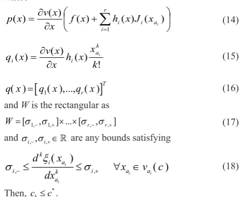
i is a parameter to be selected. Considering the specific Lyapunov function and using Taylor series and replacing the polynomial estimation in the optimization problem of theorem 1, we attain a new theorem as follow [14].where (14) + ∂ ∂ =
∑
= ri i i ai
x J x h x f x x v x p 1 ) ( ) ( ) ( ) ( ) ( (15) ! ) ( ) ( ) ( k x x h x x v x q k a i
i = ∂∂ i
(16)
[
1]
( ) ( ),..., ( )r T
q x = q x q x
and W is the rectangular as
(17) ] , [ ... ] ,
[ ,1− ,1+ × × ,− ,+
= r r
W σ σ σ σ
and σ σi,−, i,+∈ are any bounds satisfying
(18) , , ( ) ( ) i i i i k i a
i k i a a
a
d x
x v c
dx
ξ
σ
− ≤ ≤σ
+ ∀ ∈Then, *
k
c ≤c .
As explained before theorem 2 is equal to theorem 1 when we use Taylor expansion to change non-polynomial terms. It is important to know that by using Taylor series, we should also consider the effect of truncated terms into the estimation. Theorem 2 imports these truncated terms and consider an upper and lower bound for them as a rectangular in (17) which is used directly in the optimization problem (13). This theorem is proved in [14].
So, using appropriate Lyapunov function and theorem 2, we can estimate the domain of attraction of the nonlinear system with non-polynomial terms and limited perturbation as explained above. In the next section, we use this method to estimate the domain of attraction of free tumor equilibrium point of the perturbed tumor model (1) which is described in the second section.
4- domain of attraction of perturbed tumor model
First of all, we should find the equilibrium points of the model. This model has five equilibrium points that if the constants are considered as explained in section 2, we will have
(19) [ ] [ ] [ ] [ ] [ ] 1 2 3 4 5 0,0,1.66 0,0.9,0.3 0.79,0.21,0.79 0.44,0.56,0.44 1,0,1.65 T T T T T E E E E E = = = = =
From (19) it is clear that in correspondence of the equilibrium
1
E and E2, natural cells are not present. In other words in these
points malignant cells conquer the natural cells and destroy them; these points are also unstable ones. We notice them as
Dead Equilibrium Points. When the system trajectories are around the equilibrium E3 and E4, the three species of cells
are all present. We call these points Coexisting Equilibrium Points. E3 is an unstable point of this type and E4 is a stable
one. Biologically, in these points the growth of malignant cells are stopped and there is coexistence between natural cells and tumor cells. Finally the important equilibrium is E5, where in this point tumor cells are all destroyed and there exists immune and natural cells in the body. This one is called
Healthy Equilibrium Point.
From the clinical point of view E1, E2 and E3 are not important because they are all unstable points which means that if the initial conditions stand around these points, the system acts as an unstable system and the trajectories
diverge. Even though equilibrium E4 is stable and the
system’s trajectories converge, in this point malignant cells still exist in the body and the disease is not completely cured. Biologically, the most important point is E5 that is a stable
equilibrium and also the malignant cells are fully destroyed. As this point is asymptotically stable, there exists a region around this point as the domain of attraction in which if the initial condition stands in this domain, the trajectories of the system will converge to E5. This means that the disease is
completely cured. According to above explanation we are going to estimate the domain of attraction of E5 in model (1)
using theorem 2.
Since E5 is a nonzero equilibrium point, we apply the change
of variable (20) to move this equilibrium to the origin and the change of variable (21) to change the system into analytic system (20) 1 1 2 2 3 3
1
1.65
z
x
z
x
z
x
= −
=
=
−
(21) 2 2 2 xx = ′
Using these change of variables the model will be changed as
(22)
2 2 2
1 1 1 2 1 2
3
2 2 2 3 1 2 2
2
2 2
2 3
3 2 2 3 2 3
2
0.75 0.25 0.5 0.1625 0.01 ( 1.65 ) 1.65 0.2
( 0.3 )
x x x x x x
x x x x x x x
x x
x x x x x
x = − − − − = − − − − + = − − − +
Now we are going to find the appropriate Lyapunov function using Lyapunov equation (8) with linearized matrix A and
Q as follow:
(23) I Q A = − − − = , 2 . 0 0 0 0 1625 . 0 0 0 0 1
Considering these matrices and quadratic form of LF as
T
v x Px= , this function is obtained as (24) that will be met the maximum tolerance of the system against perturbation as
Fig. 1. The boundary of domain of attraction of healthy equilibrium point with equation 0.5x12+3.076x22+2.5x32-0.744=0.
In this picture axis x1 representsis represents natural cells, axis x2
explained before.
(24)
2 3 2
2 2
1 3.076 2.5 5
.
0 x x x
v= + +
After finding an appropriate LF we rewrite the state equation into the form of system (4) and use theorem 2 to estimate the domain of attraction of origin. To achieve this goal we have
(25)
2 2 2
1 1 2 1 2
3
2 2 3 1 2 2
2 2
2 3 2 3
( ) 0.75 0.25 0.5 0.1625
1.65 0.2
x x x x x
f x x x x x x x
x x x x
− − − −
= − − − −
− − −
(26)
1 2 3
2
2 3
1 1
( ) ( ) 1 , ( ) 1
1 0.01 ( 1.65 )
h x h x h x
x x
= = =
+
(27)
3 . 0 1 ) ( , 0 ) ( )
( 2
2 3
2
1 xa1 =ξ xa2 = ξ xa3 = x +
ξ
Now using Lyapunov function (24), equations (25), (26), (27), by solving optimization problem in theorem 2, we estimate the domain of attraction of healthy equilibrium point of our perturbed tumor model which its boundary equals to
(28)
744 . 0 5 . 2 076 . 3 5 .
0 2
3 2
2 2
1 + x + x =
x
In figure 1, the boundary of domain of attraction of the healthy equilibrium point with equation (28) is illustrated. It is clear that if the initial condition of the tumor stands in this domain, it will converge to the healthy equilibrium point in which the number of malignant cells are zero in it.
Finally, we can tell that we reach our goal in this paper by estimating DA of healthy equilibrium point of a nonlinear non-polynomial perturbed tumor model by using an appropriate method of computing LF to tolerate perturbation and an LMI-based method of estimating the domain of attraction of non-polynomial systems.
5- conclusions
In this paper, we propose a strategy for estimating the DA of equilibrium points for a non-polynomial perturbed system via a specific LF and an LMI optimization which is based on the usage of Taylor expansions in order to change non-polynomial terms into polynomial ones and the parameterization of their remainders inside a polytope. Moreover, choosing an appropriate Lyapunov function, by means of the linearized system so that the system can tolerate limited perturbation, is imported into the procedure of estimation. We use this technique to estimate DA of the free tumor equilibrium point of a perturbed tumor-immune model which is originally presented in [5].
Considering the healthy equilibrium point of the tumor model in which the malignant cells are completely destroyed, this method can find a region around this point that if the initial condition of disease stands in this domain, the trajectories converge to the mentioned equilibrium point. Although the dynamics of this model provide a sufficiently accurate description of the biological behavior, one could also assume that the effects of the mathematical mismatching between such model and the real one do not drive the state trajectories outside the domain of attraction of the mentioned equilibrium point. In order to obtain this goal, a procedure to select an appropriate LF is introduced in which this function assures that in limited perturbation caused by modeling error, aging
or uncertainties, the equilibrium point will not change and we may be sure that the state trajectories will not diverge. It is clear that we can also study this topic from clinical point of view. Biologically, we are interested that the tumor’s condition stays in a stable point in which the malignant cells are completely destroyed. This is the same point as healthy equilibrium point. We also want that the tumor’s trajectories with initial conditions different from free tumor equilibrium point, converge to mentioned point as far as possible. We interpret this as finding the domain of attraction of stable equilibrium point. Importance of considering perturbation from medical point of view is also explained. At last it is good to know that this topic can be a good starting point for further researches in the field of cancer treatment.
References
[1] Z. Bajzer, M. Marusic, S. Vuk-Pavlovic, “Conceptual frameworks for mathematical modeling of tumor growth dynamics,” Math. Comput. Model 23 (6) (1996) 447-455.
[2] L.G. de Pillis, A.E. Radunskaya, “A mathematical tumor model with immune resistance and drug therapy: an optimal control approach,” J. Theor. Med. 3 (2001) 79-100.
[3] L.G. de Pillis, A.E. Radunskaya, C.L. Wiseman, “A validated mathematical model of cell-mediated immune response to tumor growth,” Cancer Res. 65 (17) (2005) 7950-7958.
[4] L.G. de Pillis, W. Gu, A.E. Radunskaya, “Mixed immunotherapy and chemotherapy of tumors: modeling applications and biological interpretations,” J. Theor. Biol. 238 (4) (2006) 841-862.
[5] L.G. de Pillis, A.E. Radunskaya, “The dynamics of an optimally Controlled tumor model: A case study,” Math. Comput. Model, (37) (2003) 1221-1244.
[6] A. Merola, C. Cosentino, F. Amato, “An insight into tumor dormancy equilibrium via the analysis of its domain of attraction,” Bio. 3 (2008) 212-219.
[7] J.A. Spratt, D. von Fournier, J.S. Spratt, E.E. Weber, “Decelerating growth and human breast cancer,” Cancer 71 (1992) 2013-2019.
[8] R. Eftimie, J.L. Bramson. D.J.D. Earn, “Interactions between immune system and cancer: a brief review of non-spatial mathematical models,” Bull. Math. Biol. 73 (2011) 2-32.
[9] R. Genesio, M. Tartaglia, and A. Vicino, “On the estimation of asymptotic stability regions: State of the art and new proposals,” IEEE Transaction on Automatic Control, vol. 30, pp. 747-755, 1985.
[10] H. Chiang, M. Hirsch, and F. Wu, “Stability regions
of nonlinear autonomous dynamical systems,” IEEE Transactions on Automatic Control, vol. 33, pp. 16-27, 1988.
[11] G. Chesi, “Estimating the domain of attraction: a light LMI technique for a class of polynomial systems,” In Proceedings of the 42nd IEEE International Conference on Decision and Control, Maui, Hawaii, 2003.
control, Sidney, Australia, 2003.
[13] G. Chesi, A. Garulli, A. Tesi, A. Vicino, “LMI-based
computation of optimal quadratic Lyapunov functions for odd polynomial systems,” Int. J. Nonlinear Robust Control 15 (1) (2005) 35-49.
[14] G. Chesi, “Estimating the domain of attraction for non-polynomial systems via LMI optimization,” Automatica 45 (2009) 1536-1541.
[15] H.K. Khalil, Nonlinear systems, 3rd ed. (2001) Prentice Hall.
[16] F. Amato, C. Cosentino, A. Merola, “Estimation of the Domain of Attraction of Equilibrium Points for Quadratic Systems: Application to Tumor Stability Analysus,” American Control Conference, New York, USA, 2007, 5378-5383.
Please cite this article using:
A. Dini, M. J. Yazdanpanah, Estimation of the Domain of Attraction of Free Tumor Equilibrium Point for Perturbed Tumor Immunotherapy Model, AUT J. Elec. Eng., 50(2) (2018) 157-162.