Vol. 1, No. 3, pp. 27-34, Jan (2020)
Comparisons between Generalized Predictive
Control and Linear Controllers in Multi-Input
DC-DC Boost Converter
Mohsen Ehsani
1,†, Masood Saeidi
2, Hamid Radmanesh
3and Adib Abrishamifar
41,2,4 Department of Electrical and Computer Engineering, Iran University of Science and Technology, Tehran, Iran 3Electrical Engineering Department, Shahid Sattari Aeronautical University of Science and Technology, Tehran, Iran
In this paper, the linear state-space model of the multi-input DC-DC boost converter is obtained and based on, a linear SISO model is calculated. Model predictive control (MPC) offers a novel method of designing in the power electronic converters. The application to DC-DC converters offers real benefits because of having simple tuning technique and analytical guaranteed stability. The weakness of this converter is non minimum phase behavior. One of the methods of implementation MPC controller is Generalized Predictive Control (GPC) which is compatible with non-minimum phase systems but due to simple implementation, using of linear controller is more popular in power electronics control system. GPC has some advantage such as fast dynamic and robustness in nonlinear system however main advantage of linear controllers is its low steady state error. The main idea of this paper is the investigation performance of GPC and linear controller in the multi-input DC-DC boost converter and camper with PI controller in term of dynamic, steady-state error, and robustness and run time in a microcontroller. The resulting of this comparison is critically assessed in simulation and algorithms ruining time has been compared in microcontroller hardware.
Article Info
Keywords:
Model predictive control, DC-DC converters, Multi-Input converters, Linear controllers.
Article History:
Received 2019-01-23
Accepted 2019-08-11
I.
INTRODUCTION
The DC-DC converters play a key role in power electronic applications. They are widely used in microgrids, hybrid/electric transportation vehicles or hybrid energy systems [1]. In DC-DC power electronic converter, the DC output can be locally generated by renewable energy sources such as solar PV system, wind power generation, fuel cell, etc., and can be connected to a common DC bus [2]. Using a DC-DC Multi-Input converter to merge all of the energy sources make possible many advantages such as reduced component count, reduction in weight, control simplicity, and flexibility in the combination of sources [3]. There are various methods
for controlling the voltage and current in DC-DC converters such as PI, Fuzzy logic, Sliding Mode, MPC, each of which has its own advantages and disadvantages. In [4] proposed Sliding Mode control of DC-DC converter for wide range voltage control. Its results show using this method in wide range control is let to acceptable performance but this method in the small range make some ripple in output voltage .The conventional PI controller is used for controlling the output voltage by appropriate tuning the Kp and Ki values in PI controller, the reference signal can be sent to PWM algorithm to generate on-off time in power electronic switches [5]. The PWM controller has some advantages such as constant switching frequency, closed-loop control, small current ripple, and low sonic noise. PI controller has been vastly employed in many kinds of feedback system [6] however in recent yeses using of Model predictive control (MPC) is favorite due to its significant advantages over conventional control methods, †Corresponding Author:[email protected]
Tel: +98-9308298130,
Faculty of Electrical Engineering, Iran University of science and technology, Tehran, Iran
such as simple handling of multivariable systems, fast dynamic response, simple treatment of constraints, and easy implementable in nonlinear and linear time variation system (LTV) system [7]. MPC can be divided into Continuous Control Set (CCS)-MPC and Finite Control Set (FCS)-MPC [8]. CCS-MPC utilizes the cost functions, as well as analytical ways to provide the optimal solutions of manipulated variables that can control the power electronic switch with using the PWM or SVM modulators. According to the nature of power converter that combinations of switching states are finite, FCS-MPC uses complete enumeration method to get prediction and optimization and does not use the modulator [9]. FCS-MPC usually provides a faster response time than CCS-MPC. CCS-MPC separate the switching frequency from the controller sampling time, and by this method, the converter operates at a fixed frequency, therefore, switching loss in the converters becomes constant for these causes, CCS-MPC is more usable in industrial applications [10]. In CCS-MPC there are various control design methods based on model predictive control concepts including Dynamic Matrix Control (DMC), Model algorithmic control (MAC), Predictive Functional Control (PFC), and Generalized Predictive Control (GPC) [11]. GPC is one of the most popular predictive control algorithms developed by D. W. Clarke in 1987 [12]. GPC is one of the implemented technique MPC which uses a discrete transfer function model of the process and of the disturbance, hence, a fewer sensor is needed if compared to PFC which uses a state-space model [13].
Utilizing CARIMA model in GPC provide offset free response. GPC is suitable for non-minimum phase, open loop unstable and having variable dead time. It is capable of considering both fix and varying future set points [14].
In this paper, a linear model of the DC-DC boost converter is obtained. Linear and GPC controller are designed and their result is compared together. A key characteristic of these controllers is that guarantees stability and optimizes system response for a given DC-DC boost converter plant system.
Non-minimum phase effect in DC-DC converter cause undesired behavior in converter output voltage, therefore, using of GPC controller is proposed to avoid this phenomenon. Control algorithms are implemented in three microcontrollers for calculation the algorithms execution times.
This paper is outlined as follows: In the next section, the small signal model of the Multi-Input converter is given, and parameter design of converter is presented, then, in section III provides the PI controller design for the DC-DC converter. A full and detailed description of the automatic GPC design process is given in section IV. Later in section V simulation results are presented to compare the proposed algorithms, then this section provides the implementation results on microcontrollers are obtained for these strategies and compares them. Finally, in section VI, the main conclusions of the work are summarized.
II.
ANALYZE OF MULTI-INPUT BOOST
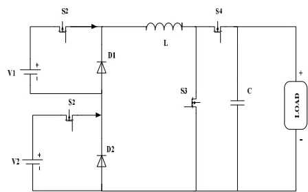
CONVERTERIn Fig. 1, the architecture of the two input DC/DC converter where source-1 and source-2 are represented by their corresponding voltage sources V1 and V2, switches S1 and S2, diodes D1 and D2, respectively. Basically, conduction of switch S1 and S2 decides the working states and supplying sources whereas conduction of switches S3 and S4 decides the operating modes (buck, boost and bidirectional).
Fig. 1.Multi-Input DC-DC boost converter schematic.
A. Multi-Input Boost Converter Model
To design the controller, it is necessary to know the system model. From the control viewpoint, the main challenge in managing the power flow between low voltage side and high voltage side is to provide a constant voltage VC when any load
disturbance appears at the output terminals [15].
In this boost converter model, there are two inputs V1and V2.
For modeling the boost converter because we want to control the output voltage, the transfer function output voltage to the output duty cycle should be obtained. Since we only need output transfer function to control the output voltage, so, it can be considered Vin=V1+V2, then according to state space in
conventional dc-dc boost converter transfer function can be extracted [16].
According to the state space model and KVL, we can obtain the following equations:
( )
( )i (t) ( )
( ) ( )
( ) ( ( ) v ( ) ( ))
( )
C
L L
L C
C C
in
C L C
C
RR
di t R R
v t
dt L L R R L R R
v t R
R i t t u t
L R R L
(1)
( ) 1
( ) v ( )
( ) ( )
( ) u(t)
( )
C
L C
C C
L C
dv t R
i t t
dt C R R C R R
R i t C R R
(2)
(t) ( ) ( ) ( ) ( )
C C
o L C L
C C C
RR R RR
v i t v t i t u t
Where, u (t) is the control input that is related to the states of the switch Q3. In that case, means the switch is ON and Q3 = 0 means is OFF. So u (t) takes a value in discrete set {0, 1}. Duty ratio d (t) indicate the average control input. By replacing
u (t) with d (t), the state-space averaged model of the DC-DC boost converter in Continuous Conduction Mode (CCM) can be obtained [17]. In equations (1) and (2), (t) and vc(t) indicates the inductor current of Land capacitor voltage of
C ,respectively. R represents load resistance, is load current, and R indicates the parasitic of capacitor and inductor respectively.
So the matrix form of state space can be written as follow:
(1 ( )) R R (1 ( )) R
( )
1
( ) ( ) ( )
( )
( ) (1 ( )) R 1
0
( ) ( )
C L L
C C L
i C
C
C C
u t R u t
di t
R R L L R R L i t
dt v
L v t
dv t u t
R R L R R L
dt (4)
The input and output voltage are define v (t), and v (t) respectively.
The equations of states variables ( ), contain time-varying quantities which cause non-linearity in the system. To obtain a linearized state equation of the system, small signal ac perturbations are superimposed in duty cycles, voltages, and currents. Therefore time-varying quantities along with a perturbation are expressed as:
̃ = (t) − , (t) = (t) − , d̃(t) = d(t) − D , (t) = (t) – where the uppercase letters represent the nominal steady state values. By Laplace transform of the obtained linear state-space
Model, transfer function output to duty cycle can be obtained as follows:
2 2
3
(1 ) (1 ) ( )( )
1 (s)
o o C C L
dout
CR S R D R R R LS
v V
G
d D
(5)
( ) (1 D) (1 ) (1 ( )
( )( )(1 ( ) )
C C
C L C
s R R D R C R R S
R R R LS C R R S
(6) In this section we want to design the parts of DC-DC converter. In order to operate the converter in CCS mode the inductance is calculated such that the inductor current flows continuously and never falls to zero [18]. Thus, L is given by 2 min (1 ) 2
D DR
L
f
(7)
Where Lmin is the minimum inductance, D is duty cycles, R
is output resistance, and f is the switching frequency of switch. The output capacitance to give the desired output voltage ripple is given by min r D C RfV (8)
Where is the minimum capacitance and is output voltage ripple factor. Can be expressed as: o r o V V V (9) According to output voltage equation in boost converter, for =70V duty cycle is d=0.485.
From equation (7) and (8), Lmin=0.16mH and Cmin=9.7µF.
In this paper we have considered the value of L and C are 390µH and 100µF respectively, therefore system transfer function is calculated as follow:
6
2 5 4
92 10 0.12 9.8 10 6.6 10
d S G s S S (10)
III.
LINEAR CONTROLLER DESIGN
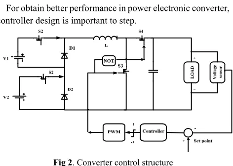
For obtain better performance in power electronic converter, controller design is important to step.
Fig 2. Converter control structure
In past decades, using of linear controllers are conventional and practical in industrial systems. The implement of the linear controller has some advantages such as linear controllers are used often in many industries. These type of controllers have some advantages such as simple design, low-cost implementation, and explicit stability proof also use of linear controllers have some disadvantages as dependence controller parameters to system operation point, the unsuitable response in time delay system and frailty against disturbances [19]. To design the linear controller, defin the transfer function from duty cycle D (manipulated variable) to output voltage (controlled variable) is necessary.
In control structure, use of PWM modulator with 20 kHz switching frequency, the controller generates a reference signal for the modulator. The improved PI controller has been proposed in this system because this type of controller can both improve the response speed, stability margin and according to the existence of the integrator in the controller structure, the steady-state error will be decreased. The structure of the controller is shown in the Fig. (6).
controller design. Bode diagram of the transfer function of Eq. (10) is depicted in Fig 3
Fig. 3. Bode diagram of transfer function
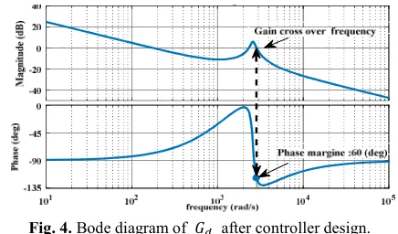
The system phase margin is 89.9(deg) which is not appropriate for industrial systems [20]. Higher phase margin, because the slower dynamic response, with the appropriate controller design, the system phase margin should be ranged in 30-65 degrees.
The PI controller in practical implementation is express as follow [20]:
( i)
p
k PI controller k e s
s
(11)
System close loop transfer function by utilizing of mason method is define as follow [20]:
Vout kpkT s
Duty cycle
(12)Where, ∆ is system characteristic equation, is route gain and ∆ is system characteristic equation cofactor. Fig. 4 shows bode diagram of after controller design.
With using of MATLAB /SIMULINK software, controller parameter are tuning with purpose of raise time and over shot percentage reduction. The simulation result is shown in section V.
Fig. 4. Bode diagram of after controller design.
IV.
MODEL PREDICTIVE CONTROL
Model Predictive Control (MPC) is an advanced control method used in the industrial process from the 1980s. The dynamic model of the system is used in the MPC controller. By solving open-loop optimization problem optimal control move is calculated on-line at each sampling time.The optimal sequence of the manipulated variable is computed over the control horizon based on the current system. Only the first control move is applied to the system. This is the contrary to the pre-computed control law such as PI control where the closed-loop operation is employed [20].
Features such as high dynamics, the capability to using in the unstable system and the possibility of consideration constraint in controller design. The main disadvantages are the requirement of the accurate model and possible instability when the prediction horizon is not selected well. In power electronics, the MPC is divided into two classes according to the control set Finite Control Set (FCS) MPC and Continuous Control Set (CCS) MPC. The first one does not need a modulator and has a variable switching frequency. The second one uses a modulator and thus uses a constant switching frequency. Each one of these approaches has its advantages. The CCS MPC was used for this work as it can be easily compared to the PI controller.
The MPC is a multivariable control algorithm. The calculation of the optimal control move is based on solving the optimization problem defined by a cost function [21].
1
2 1
2
1 , ,
[Δ
ˆ |
1
p
c
N
p c j N
N
j
J N N N j y t j t w t j
j u t j
(13)
Where, is prediction horizon, control horizon, model delayed, Δ control signal, ( ) model output, w (t) reference set point and ( ), ( ) are the weight factors.
CCS-MPC controller is implemented by 4 forms that consist of Dynamic matrix control (DMC), Model algorithmic control (MAC), Predictive functional control (PFC) and Generalized predictive control (GPC) [22]. In this paper we are used GPC format because its formulation is based on using system transfer function.
For tuning parameters of the MPC controller, prediction horizon in oscillating systems should be noted that using of appropriate criterion leads to acceptable and implementable design. If the control horizon of the system model be selected as long range, the calculation rate of the system is decreased and complexity is extremely increased.
1
1 11 1
429.72 208.32 1 .212 .842
d
Z Z
G Z
Z Z
(14)
Mostly, in GPC method, controlled auto regressive integrated moving average (CARIMA) model type is used that is based on the transfer function of the plant according to discrete time structure,
This transfer function often describe as a fraction two polynomial
1 1 1
1 0 1 2
1 1
1
1 2
1
nb nb
d na
na
B Z b b Z b Z b Z
G Z
a Z a Z a Z
A Z
(15)
The equation of CARIMA model can be written as following:
1
1
1
t A Z y t B Z u td C Z
(16)
The last term in Eq. (16) shows the disturbance effect. If
( ) is white noise, the polynomial can be set to 1. So the equation can be simplified to:
1
1
1
tA Z y t B Z u t
(17)
For provide a predictor, the following Diophantine equation is expressed as:
1
1
1
1 j
j j
E Z A Z Z F Z
(18)
By definition ( ) = ∆ ( ) where Eq.(17) Can be written as:
1
1
1 E Zj Z F Zj j
(19)
Through dividing 1⁄ ( ) two terms the remainder factorized as ( ) . The quotient is the polynomial ( ). So, The degree of ( ) is j-1 which
= ,there for ( ) and ( ) can be defined as:
1 1 2 ( 1)
,0 ,1 ,2 , j 1
( ) ... j
j j j j j
E Z e e Z e Z e Z
(20)
1 1 2
,0 ,1 ,2 ,
( ) ...f na
j j j j j na
F Z f f Z e Z Z
(21)
The best prediction for output y is:
1
1
y t j G Zj U t j 1 F Zj y t
(22)
In which: = ( ) ( )
In Eq. (21) The term ( )∆ ( + − 1) including two part, past and future. Sum of the past output term with ( )
is called free response (f) and system response to future value is force response.
1
1
y t j 1
j j j j
F G G Z U t j F Z y t (23)
In this paper assume no constraint is excitant exist in the system. By minimizing Eq. (13) the optimal control signal is calculated as following:
2 T 2 T
j
G G I U G f w
U
(24)
Where:
T
1 T
U G GI G wf (25)
In before equation, represents the free response of the system, λ the weighting factor and the reference trajectory.
V.
SIMULATION RESULTS
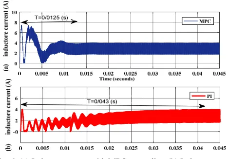
In this section compression between MPC and PI controllers are investigated. Output voltage when the converter load is 100W is showing in Fig 5 . From Fig 5,6 is deduced that the MPC controller is faster (about 4 times) than PI controller and its dynamic response is smooth but have some overshoot in its response. From point of the steady state, both PI and MPC have the same response. For some application such as a protection
system which requires fast dynamic MPC is the proper choice. In Fig. 6 output current is shown that once again indicate MPC is faster dynamic compared with PI and has some overshoot.
TABLE I
DC-DC CONVERTER PARAMETERS VALUE Value
Unit Parameter
.16 mH
L
9.7 C
20 kHz
12 volt
24 volt
70 volt
Fig. 5. Converter output voltage in 100W load.
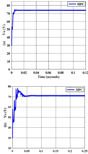
Fig. 6. (a) Inductor current with MPC controller, (b) Inductor current with PI controller
A load step change test is used to verify the effect of uncertainties in the load on the output voltage tracking capabilities. In t = 0.1 S load is increased by change the load resistance from
Fig. 7. (a) -Output voltage with 70% load increase by MPC method, (b)- Output voltage with 70% load increase by PI
Fig. 8 shows output reference voltage when the load is twice increased by changing the load resistance from 50 Ω to 25 Ω (50% load increase). Due to this change in t = 0.1s, both controllers have same undershoot and speed but the MPC controller illustrate less transient oscillation to reach steady state compared with PI controller.
Fig. 8. (a) Output voltage with 50% load increase by MPC method, (b) Output voltage with 50% load increase by PI method
Now, the input change effect on output voltage will be investigated. Fig. 9 illustrates the output voltage when the input sources work at 80% nominal value. As can be seen, The MPC is faster about 3.5 times. Unlike PI controller at t = 0.004s MPC demonstrate an overshoot.
Fig. 9. (a)- Output voltage with 80% sources nominal voltage in MPC method, (b)-Output voltage with 80% sources nominal voltage in PI method
Now, for investigation effect of sample time on the output voltage of the MPC controller, it could be 10 times increased and decreased. At first, sample time decrease to (Ts= 0.000056 s) and after sample time is increased reach to (Ts = 0.0056 s) . As shown in Fig 10, in first case, output voltage response has fast dynamic but steady state error is increased because in this condition system tends to instability. According to Fig 10, in this case, output voltage response has a slow dynamic but steady state error is decreased and it close to the reference value.
Fig 10. Output voltage when sample time is 10 times increased and decreased. (a) Ts = 0.000056s, (b) Ts = 0.0056s.
Runtime Evaluation
For illustrating the computational complexity of linear and MPC controllers, their runtime when are implemented in the microcontroller is compared together. This algorithm implantation is developed by using the MATLAB/SIMULINK code generation method.
Fig. 11. Code generation procedure in MATLAB
In this paper TMS320F28335 with 150MHZ CPU clock, ARM cortex-M3 with 84 MHZ CPU clock and AVR atmega32 with 16 MHZ CPU clock are selected. Table II is showing runtime results in different microcontrollers. From this table, it is clear that the linear controller is implementable in all three
(
a)
V
o
(V
of the controller but GPC has the limitation in AVR microcontroller. From this table is understandable that if the GPC controller tuning parameter is changed, it affect the runtime of this algorithm.
TABLE II
CONTROL ALGORITHMS RUNTIME IN MICROCONTROLLER
Avr(ATmega32)
Arm(Cortex-M3) Tms(
f28335)
19.45 8.12
3.66 Linear
controller (PI)
25.82 10.78
4.86 Gpc ( =
25 , =
10, = 2)
65.72 27.44
12.45 Gpc ( =
2.5 , =
10, = 5)
74.56 30.15
14.32 Gpc ( =
2.5 , =
15, = 2)
VI.
CONCLUSIONS
In this paper, two strong candidate controllers are presented for voltage control of the multi-input boost converter. The transfer function of the output voltage to duty cycle is used to controller design for both GPC and PI controller. From the simulation result, the two control schemes exhibit good performance Keeping all system variable within nominal rate, i.e., output voltage and its ripple and inputs current. The results illustrate that the GPC controller has a very fast dynamic response and have robustness than PI controller again changing system load and parameter mismatch. Rather than GPC controller, PI has less output voltage steady state error. Approximately same output voltage ripple has been obtained by the two control scheme, however, by investigating the computational burden in microcontrollers it can be seen the PI controller consume low processing time and it can be implemented with lower cost microcontroller.
R
EFERENCES[1] K. Varesi, S. Hosseini, M. Sabahi and E. Babaei, “Modular non-isolated multi-input high step-up dc–dc converter with reduced normalised voltage stress and component count”, IET Power Electronics, vol. 11, no. 6, pp. 1092-1100, 2018. [2] T. Taufik, K. Htoo and G. Larson, “Multiple-input bridge converter for connecting multiple renewable energy sources to a DC system”, 2016 Future Technologies Conference (FTC), 2016.
[3] V. Karthikeyan and R. Gupta, “Multiple-Input Configuration of Isolated Bidirectional DC–DC Converter for Power Flow Control in Combinational Battery Storage”, IEEE Transactions on Industrial Informatics, vol. 14, no. 1, pp. 2-11, 2018.
[4] A. Taheri, N. Asgari, “ Sliding Mode Control of LLC Resonant DC-DC Converter for Wide Output Voltage
Range in Battery Charging” International Journal of Industrial Electronics, Control and Optimization (IECO), Vol 2, Issue 2, , PP 127-136 spring 2019.
[5] R.Nagarajan, J.Chandramohan, S.Sathishkumar, S.Anantharaj, G.Jayakumar, M.Visnukumar and R.Viswanathan, “Implementation of PI Controller for Boost Converter in PV System,” International Journal of Advanced Research in Management, Architecture, Technology and Engineering (IJARMATE). Vol.11, Issue.XII, pp. 6-10, December. 2016.
[6] A. Urtasun and D. D. Lu, “Control of a Single-Switch Two-Input Buck Converter for MPPT of Two PV Strings,” inIEEE Transactions on Industrial Electronics, vol. 62, no. 11, pp. 7051-7060, Nov. 2015.
[7] Z. Wang, Z. Zheng, Y. Li, B. Fan and G. Li, “Predictive current control for induction motor using online optimization algorithm with constrains”, 2017 IEEE Energy Conversion Congress and Exposition (ECCE), 2017. [8] J. Rodriguez, M. P. Kazmierkowski, J. R. Espinoza, P.
Zanchetta, H. Abu-Rub, H. A. Young, and C. A. Rojas, “State of the Art of Finite Control Set Model Predictive Control in Power Electronics,” Industrial Informatics, IEEE Transactions on, vol. 9, pp. 1003-1016, May 2013.
[9] L. Cheng et al., “Model Predictive Control for DC–DC Boost Converters With Reduced-Prediction Horizon and Constant Switching Frequency”, IEEE Transactions on Power Electronics, vol. 33, no. 10, pp. 9064-9075, 2018. [10] L. Cavanini, G. Cimini, G. Ippoliti and A. Bemporad,
“Model predictive control for pre-compensated voltage mode controlled DC–DC converters”, IET Control Theory & Applications, vol. 11, no. 15, pp. 2514-2520, 2017. [11] S.Holkar & L.Waghmare,. “An overview of model
predictive control”, Internationa Journal of Control and Automation, 3, 47–64, 2010.
[12] D.W.Clarke, C. Mohtadi and P. S. Tuffs, “Generalized Predictive Control -Part I. The Basic Algorithm”,Automatica, Vol. 23 (Issue 2), pp. 137-148, 1987.
[13] D. Lima, V. Montagner and L. Maccari, “Generalized predictive control with harmonic rejection applied to a grid-connected inverter with LCL filter”, 2017 Brazilian Power Electronics Conference (COBEP), 2017.
[14] A. Linder and R. Kennel, “Model Predictive Control for Electrical Drives”, IEEE 36th Conference on Power Electronics Specialists, 2005.
[15] L. Cheng, P. Acuna, R. Aguilera, M. Ciobotaru and J. Jiang, “Model predictive control for DC-DC boost converters with constant switching frequency”, 2016 IEEE 2nd Annual Southern Power Electronics Conference (SPEC), 2016. [16] T. Kobaku, S. Patwardhan and V. Agarwal, “Experimental
Evaluation of Internal Model Control Scheme on a DC–DC Boost Converter Exhibiting Non minimum Phase Behavior”, IEEE Transactions on Power Electronics, vol. 32, no. 11, pp. 8880-8891, 2017.
[17] R. Leyva, I. Queinnec, C. Olalla, “Robust Linear Control of DC-DC Converters: A Practical Approach to the Synthesis of Robust Controllers”, VDM Verlag Dr. Müller, 2010. [18]
S. Masri and P. Chan, “Design and development of a DC-DC boost converter with constant output voltage”, 2010 International Conference on Intelligent and Advanced Systems, 2010.
using fuzzy logic algorithm," in Electronics Letters, vol. 52, no. 15, pp. 1327-1329, 7 21 2016.
[20] L. Dai, Y. Xia, M. Fu, M. S. Mahmound, “Discrete-time model predictive control”, in Proc. Advances in Discrete Time Systems, Intech, pp. 77–116, 2012.
[21] J. Rodriquez, P. Cortes, “Predictive Control of Power Converters and Electrical Drives”, Wiley-IEEE Press, p. 230, 2012.
[22] Eduardo F. Camacho, Carlos Bordons, “Model Predictive Control”, Springer publication, London, 2007.
-energy-consumption-since-1820-in-charts, 2014.
Mohsen Ehsani was born in BandarAbbass, Iran. He received his B.S. degree in Electrical Engineering from Shiraz University of Technology (SUTECH), Shiraz, Iran, in 2015, M.Sc. degree in Electrical Engineering from Iran University of Science and Technology (IUST), Tehran, Iran, in 2019. Iran. His current research interests include DC-DC converters and Predictive controllers.
Masood Saeidiwas born in 1994. He received the B.Sc. degree in electrical engineering from Shahid Beheshti University, Tehran, Iran in 2016 and currently, is the M.Sc. of electrical engineering in Iran University of Science and Technology, Tehran. iran since 2016 . His main interesting activity is related to power electronic converter modeling, model predictive control applications in power electronics, electrical machine control, power system control and renewable energy.
Hamid Radmanesh (M’15) was born in 1981. He received the B.Sc. degree in electrical engineering from Malek-Ashtar University of Technology, Tehran, Iran, in 2006, the M.Sc. degree in electrical Engineering from Shahed University, Tehran, in 2009, and the Ph.D. degree in electrical engineering from Amirkabir University of Technology (AUT), Tehran, in 2015. He has authored more than 100 published technical papers and has been involved in several industrial projects and educational programs in the fields of power electronics and power systems. His research interests include transient in power system, renewable energy, power quality, HVdc transmission systems, and more-electrical aircraft.