Bayesian Quantitative Trait Loci Mapping for Multiple Traits

DOI: 10.1534/genetics.108.088427

Bayesian Quantitative Trait Loci Mapping for Multiple Traits

Samprit Banerjee,* Brian S. Yandell

†

_{and Neng jun Yi*}

,1

*Department of Biostatistics, Section on Statistical Genetics, University of Alabama, Birmingham, Alabama 35294 and†Departments of Statistics, Horticulture and Biostatistics and Medical Informatics, University of Wisconsin, Madison, Wisconsin 53706

Manuscript received February 22, 2008 Accepted for publication June 15, 2008

ABSTRACT

Most quantitative trait loci (QTL) mapping experiments typically collect phenotypic data on multiple correlated complex traits. However, there is a lack of a comprehensive genomewide mapping strategy for correlated traits in the literature. We develop Bayesian multiple-QTL mapping methods for correlated continuous traits using two multivariate models: one that assumes the same genetic model for all traits, the traditional multivariate model, and the other known as the seemingly unrelated regression (SUR) model that allows different genetic models for different traits. We develop computationally efficient Markov chain Monte Carlo (MCMC) algorithms for performing joint analysis. We conduct extensive simulation studies to assess the performance of the proposed methods and to compare with the conventional single-trait model. Our methods have been implemented in the freely available package R/qtlbim (http://www.qtlbim.org), which greatly facilitates the general usage of the Bayesian methodology for unraveling the genetic architecture of complex traits.

C

OMPLEX traits involve effects of a multitude of genes in an interacting network. Mapping quan-titative trait loci (QTL) means inferring the genetic architecture (number of genes, their positions, and their effects) underlying these complex traits. The QTL mapping problem has several salient features: first, the predictor variables in the regression (the genotypes of QTL) are not observed; second, it is really a model se-lection problem as there are typically thousands of loci to choose from; and third, the genomic loci on the same chromosome are correlated. Much has been done in this regard, especially in the univariate case (e.g., Lander and Botstein1989; Jiangand Zeng1997; Bromanand Speed2002). Bayesian methods have been very success-ful in the QTL mapping framework (Satagopan and Yandell 1996; Yi and Xu 2002; Yiet al. 2003, 2005, 2007; Yi2004); see a recent review by Yiand Shriner (2008).

Most of these methods are applicable to mapping QTL for a single trait. However, in QTL experiments typically data on more than one trait are collected and, more often than not, they are correlated. It seems nat-ural to jointly analyze these correlated traits. There are two distinct advantages for jointly analyzing correlated traits: including information from all traits can increase the power to detect QTL and the precision of the estimated QTL effects. Biologically, it is imperative to jointly analyze correlated traits to answer questions like pleiotropy (one gene influencing more than one trait)

and/or close linkage (different QTL physically close to each other influencing the traits). Testing these hypoth-eses is key to understanding the underlying biochemical pathways causing complex traits, which is the ultimate goal of QTL mapping.

Several methods have been developed to jointly analyze multiple correlated traits. Some of them use a maximum-likelihood-based approach ( Jiangand Zeng 1995; Jackson et al. 1999; Williams et al. 1999a,b; Vieiraet al.2000; Huangand Jiang2003; Lundet al. 2003; Xuet al.2005) or a least-squares approach (Knott and Haley2000; Hackett et al.2001). Most of these methods involve a single-QTL model or at most very few QTL. A problem with the likelihood-based approach is that with increasing complexity, due to the increase in the number of parameters to be estimated, the increase in degrees of freedom of the test statistic can restrain its practical use when the number of traits is large (Mangin

et al.1998). As a result, the advantage of joint analysis is lost over single-trait analysis. Another approach for joint analysis is to use a dimension reduction technique, namely, principal component analysis (PCA) or discrim-inant analysis (DA) or using canonical variables associ-ated with the traits (Manginet al.1998; Ma¨ hleret al. 2002; Gilbertand LeRoy2003, 2004), and then use the linear combination of traits to map QTL. The problem with this approach is that linear combinations of traits are not biologically interpretable and can cause spurious linkages (Ma¨ hleret al.2002; Gilbertand Le Roy2003). Gilbertand LeRoy(2003) compared the performance of PCA, DA, and the multivariate model in a full-sib family and half-sib families under differ-1_{Corresponding author: Department of Biostatistics, University of}

Alabama, Birmingham, AL 35294-0022. E-mail: [email protected]

ent scenarios. Lange and Whittaker (2001) use a nonparametric generalized estimating equations ap-proach to multivariate QTL mapping.

Meuwissen and Goddard (2004) used a Markov chain Monte Carlo (MCMC) algorithm to map QTL, using linkage disequilibrium and linkage information for multiple-traits data. Recently, Liu et al.(2007) de-veloped a Bayesian approach to map QTL for a com-bination of normal and ordinal traits in a full-sib design based on the variance components approach. They used a reversible-jump (RJ) MCMC to estimate the unknown number of QTL. The problem with RJ-MCMC is that increased complexity drastically increases the computa-tional burden, rendering it unsuitable for genomewide scans where typically thousands of positions are scanned for a putative QTL. Another major challenge is to ascertain convergence of the RJ sampler and obtain a rapidly converging sampler (Yi 2004). Yang and Xu (2007) extended the Bayesian shrinkage analysis with a fixed-interval approach (Wang et al. 2005), where a QTL is placed in each marker interval, to a moving-interval approach, where the position of a QTL can be searched in a range that covers many marker intervals for dynamic/longitudinal traits using a Legendre poly-nomial. Their method, however, focuses on the study of the growth trajectory of time-dependent or repeated-measures types of outcomes (called dynamic traits) and is very different from our approach.

All the multivariate methods mentioned here use the traditional multivariate regression model, which as-sumes the same genetic model for all traits. However, almost all correlated traits are actually affected to some extent by a different multilocus network. To capture this facet of multiple traits we use the so-called ‘‘seemingly unrelated regression’’ (SUR) model (Zellner 1962), which allows each trait to have a different set of QTL. Verzilliet al.(2005) implemented a Bayesian version of SUR using RJ-MCMC to jointly analyze multiple corre-lated traits with SNP data in a human population. They found it difficult ‘‘to deal with very many loci’’ and restricted attention to only 12 SNPs. Their method appears unsuitable to genomewide scans.

In the literature of joint analysis for QTL mapping, there is a lack of comprehensive genomewide strategies to map multiple pleiotropic and nonpleiotropic QTL. In this article, we extend the composite model space approach of Yi(2004) to jointly analyze multiple cor-related continuous traits. Multiple traits are modeled using novel QTL SUR models that enable us to detect either the same or different QTL for different traits, facilitating the separation of pleiotropy and close link-age. The QTL SUR models include the traditional multi-variate model and the single trait-by-trait model as special cases. We develop computationally efficient MCMC algorithms for performing joint analysis. Fi-nally, we conduct extensive simulation studies to assess the performance of the proposed methods.

BAYESIAN MODELING OF MULTIPLE QTL FOR MULTIPLE TRAITS

QTL SUR models: We focus our attention on

experimental crosses derived from two inbred lines. Observed data in QTL mapping consist of phenotypic values of complex traits and molecular marker data. We extend the composite model space approach of Yi (2004) to jointly analyze multiple correlated continuous traits. We assume that the marker data include not only the marker genotypes but also the genomic positions of the markers. We approximate positions for all possible QTL using a partition of the entire genome into evenly spaced loci, including all observed markers and addi-tional loci (called pseudomarkers) between flanking markers (Sen and Churchill 2001; Yi et al. 2005). Inserting pseudomarkers enables us to detect potential QTL within the marker intervals, but introduces a special statistical problem; i.e., QTL genotypes are unobserved. Before mapping QTL, we calculate the probabilities of genotypes at these preset loci given the observed marker data as priors of QTL genotypes in our Bayesian framework.

The actual number of detectable QTL for each trait in a particular experiment is unknown, but usually not too large. We employ a composite model space approach (Yi 2004; Yiet al.2005) and consider at mostLpossible loci. The upper bound L is larger than the number of detectable QTL with high probability for a given data set and can be set on the basis of the initial analyses using conventional mapping methods on each trait (Yi2004; Yi

et al.2005). Conditioning on the genotypes at theseLloci for all individuals, the phenotypic valuesytifor individual ion traittcan be expressed as a linear regression,

yti¼mt1Xtibt1eti; t¼1;2; ;T; i¼1;2; ;n;

ð1Þ

where T and n represent the numbers of traits and individuals, respectively, the subscriptstandirepresent thetth trait and theith individual, respectively,mtis the overall mean for traitt,Xtiis the row vector of the main-effect predictors ofLloci, determined from the geno-types by using a particular genetic model [we use the Cockerham genetic model, although other genetic models are possible (Kao and Zeng2002; Zenget al. 2005)],btis the vector of all main effects forLloci of traitt, and the vector of residual errors across traits,ei, is independent and normal with mean0and covariance matrix S; i.e., eiNTð0;SÞ. Thus, the residual errors are independent among individuals, but are correlated among traits within individuals. The above equations can be rewritten as

y_iNTðm1Xib;SÞ; i¼1; 2; ;n; ð2Þ

can include a large number of effects, many of which are irrelevant to modeling the phenotype and should be excluded from the model. We use an unobserved vector of indictor variables gt¼ ðgt1;gt2; ;gtj; Þ to indicate which effects bt ¼ ðbt1;bt2; ;btj; Þ9 are included in (g_tj¼1) or excluded from (g_tj ¼0) the model for the tth trait. We denote the genomic positions of L loci for trait t by the vector lt ¼

ðlt1; ;ltLÞ. The vector ðlt;gtÞ thus determines the genetic architecture of the tth trait, i.e., the actual number of QTL, their positions, and the activity of the associated genetic effects. Our goal is to infer the pos-terior distribution ofðlt;gtÞand estimate the associated genetic effects.

Model (1) or (2) uses trait-specific effect predictors

ðXtiÞ, positionsðltÞ, and indicator variablesðgtÞ, allow-ing each trait to have a different set of QTL or a different genetic model. Therefore, models for different traits seem unrelated, but actually are related through corre-lated residual errors (or observed phenotypes) or the genotypes of linked QTL. Hereafter, we refer the above model as the QTL SUR model. We consider two different SUR models. In the first model as described above, different traits can have different sets of Lloci

ðltÞ and thus different indicator variables ðgtÞ and predictorsðXtiÞ. The second SUR model uses the same set of L loci, i.e., l1¼ ¼lTbl and thus

X1i¼ ¼XTi, but different indicator variables for different traits. We denote these two SUR models by SUR modeling with different loci used for all traits (SURd) and SUR modeling with the same loci used for all traits (SURs). Note that both QTL SUR models include two existing models as special cases, the univariate single-trait approach (STA) where the re-sidual errors are unrelated, i.e., S¼I, and the tradi-tional multivariate (TMV) model where all traits have the same set of loci and the same indicator variables,i.e., l1¼ ¼lT,X1i¼ ¼XTi, andg1¼ ¼gT.

Prior distributions: To complete Bayesian modeling

of QTL SUR, we need to specify prior distributions for all unknowns. We describe the prior distributions for the model SURd in detail (appendix a), which can be easily adapted to the models SURs and TMV. For SURd, unknowns include the positions l¼ ðl1; ;lTÞ, in-dicator variablesg¼ ðg₁; ;g_TÞ, main effectsb, over-all meanm, residual covariance matrixS, and genotypes g¼ ðg_tiq;t ¼1; ;T;i¼1; ;n;q¼1; ;LÞ, where g_tiq is the genotype of individualifor traittat locusq.

As described in the previous section, the prior ong_tiq is the probability of the genotype given the observed marker data. For computational reasons, we directly work on the inverse matrix S1 instead ofS (see the next section andappendix b). The prior forS1can be taken to be the commonly used noninformative prior; i.e.,pðS1Þ jS1jð11TÞ=2(see Gelmanet al.2004). We assume that the unknownsðlt;gt;mt;btÞare indepen-dent among the traits. For each trait, the priors on

ðlt;gt;mt;btÞcan be specified as in Yiet al.(2005, 2007), which we describe inappendix a.

MARKOV CHAIN MONTE CARLO ALGORITHM

We fit the models using the MCMC algorithm, applied to the joint posterior density of all the un-knownsðm;b;s;S1;g;l;gÞ. The joint posterior distri-bution can be expressed as

pðm;b;s;S1_;g;l;gjyÞ

}Y

n

i¼1

pðy_ijm;b;S1;Xi;gÞ pðg;m;b;s;S1;l;gÞ;

ð3Þ

where the likelihoodpðy_ijm;b;S1;Xi;gÞis defined by model (2), and the prior pðg;m;b;s;S1;l;gÞ is de-scribed in the last section and appendix a, and the augmentation with hyperparameters s presents the prior variances for the effects b (Yi et al. 2007; see appendix a). For notational convenience, we suppress the dependence on the observed marker data here and afterward.

The joint posterior distribution can be simulated using the Gibbs sampler and Metropolis algorithm, alternately updating each unknown conditional on all other param-eters and the observed data. We show all the conditional distributions inappendix b. Conditional updates ofm,b, s, andS1are the same for the models SURd, SURs, and TMV. However, conditional updates of g,l, andg are illustrated only for the SURd model, which can be easily adapted to the SURs and TMV models (seeappendix b). Below, we describe our algorithm, with more details on steps for unknowns where the method involves explicit extension for multiple correlated traits.

A commonly used updating scheme for the overall means and the coefficients is performed by updating jointlymandbfor all traits (see Smithand Kohn2000; Griffiths 2001; Verzilli et al. 2005). This scheme requires large matrix operations at each simulation iteration, resulting in prohibitive computational burden for genomewide multiple-QTL analysis. We have de-veloped a pure Gibbs sampler to update one parameter at a time: for eachtandj, we samplem_tandb_tjfrom their conditional posterior distributions, respectively, which are normal distributions (see Equations B1 and B2 in appendix b). This one-at-a-time algorithm never requires matrix operations and is computationally very efficient. Note that ifg_tj ¼0, we do not need to sampleb_tj.

The variance parameters s2

tk are updated one at a time: for each t and k, the conditional posterior distribution of s2

tk is a scaled inverse x

2_{-distribution}

stan-dard Wishart distribution, and thus both the Gibbs sampler and the Metropolis algorithm can be applied to updateS1 (see Equations B4 and B5).

The genotypes are usually updated one at a time from the conditional posterior distributions. If locus q is included in the model and the genotype gtiq is not observed, the conditional posterior distribution ofgtiq is a simple multinomial (or binomial) distribution and thus can be sampled directly (see Equation B6); other-wise, we do not need to samplegtiq. The positionslare also updated one at a time. As above, we need to update only those loci that are included in the current model. The conditional posterior distribution of (ltq,g_tq) is not a standard distribution, and thus a Metropolis algorithm is needed to update (ltq,g_tq) (see Equations B7 and B8 inappendix b).

The indicator variables gare also updated one at a time. The binary indicator variables g_tj for the SUR models have independently binomial conditional pos-terior distributions (see Equations B9 and B12 in appendix b). At each iteration, therefore, the Gibbs sampler can be used to generate each indicator from its conditional posterior. However, for the QTL SUR models, using the Gibbs samplers is computationally demanding because the SUR models containT times the number of indicators as a single-trait model and most of the indicators are zero. To speed up the

rithm we extend the Metropolis–Hastings (MH) algo-rithm proposed by Yi _{et al.} (2007) to the QTL SUR models in a natural way (see Equation B11). This MH algorithm can be easily adapted to the TMV model.

SUMMARIZING AND INTERPRETING THE POSTERIOR SAMPLES

Assessing the convergence and mixing behavior of any MCMC algorithm is somewhat difficult to ascertain and it is intensified for a high-dimensional problem. Several methods have been developed so far; many are implemented in R/coda (Plummeret al. 2004), an R package providing an object-based infrastructure for analyzing output of MCMC simulations and performing convergence diagnostics.

The posterior samples generated by the above MCMC algorithm contain all available information about the unknowns in the QTL SUR and thus the genetic archi-tecture of the multiple traits. The vector (lt;gt) deter-mines the number of QTL, their positions, and the main effects of QTL, for the tth trait and hence identifies its genetic architecture. The posterior inclusion proba-bility for each locus is estimated as its frequency in the posterior samples. The larger the effect size is for a locus, the more frequently the locus is sampled. Taking the prior probability into consideration, we use Bayes factors (BF) to show evidence for inclusion against exclusion of a locus. Bayes factors are calculated on the basis of the idea of model averaging. The Bayes factor of thejth locus for the tth trait can be represented as the ratio of the posterior to prior odds of selecting that particular locus. Model averaging accounts for model uncertainty and hence provides more robust inference compared to a single ‘‘best’’ model approach (Rafteryet al.1997; Ball 2001; Sillanpa¨ a¨and Corander2002).

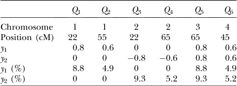
Since the information about correlation between multiple traits is taken into account, the proposed QTL SUR model is expected to increase the probability TABLE 1

True positions of six QTL, their effects, and heritabilities

Q1 Q2 Q3 Q4 Q5 Q6

Chromosome 1 1 2 2 3 4

Position (cM) 22 55 22 65 65 45

y1 0.8 0.6 0 0 0.8 0.6

y2 0 0 0.8 0.6 0.8 0.6

y1(%) 8.8 4.9 0 0 8.8 4.9

y2(%) 0 0 9.3 5.2 9.3 5.2

TABLE 2

Average correct and incorrect QTL detected for traitsy1(first row) andy2(second row)

Correct Extraneous

ðn;r_y1y2Þ STA TMV SURs SURd STA TMV SURs SURd

(100, 0.5) 0.65 0.8 0.67 0.64 0.7 1.34 0.45 0.65

0.74 0.78 0.64 0.81 0.39 1.36 0.26 0.59

(100, 0.8) 0.34 1.01 1.02 0.97 0.24 1.85 0.75 0.54

0.78 1.07 1.3 1.21 0.71 1.72 0.84 0.78

(200, 0.5) 1.69 2.13 2.12 1.78 1.06 2.53 0.78 1.02

1.76 2.2 2.16 1.67 0.63 2.55 0.78 0.69

(200, 0.8) 1.51 2.6 2.56 2.24 0.63 2.92 0.73 0.72

1.75 2.61 2.66 2.4 0.96 2.96 0.84 0.8

(500, 0.5) 3.54 3.72 3.76 3.66 1.01 3.1 0.83 1.22

3.59 3.79 3.75 3.56 0.76 3.07 0.67 0.88

(500, 0.8) 3.55 3.81 3.78 3.67 1.1 3.14 1.03 1.01

of detecting QTL, especially weak-effect QTL. More importantly, the QTL SUR model allows for a statistically rigorous procedure to test a number of biologically important questions involving multiple traits, such as pleiotropy and pleiotropyvs. close linkage. To test if the jth locus is a pleiotropic QTL we considered all models that include thejth locus for all traits (i.e., all models withg_tj ¼1 for all t) and compute the joint posterior inclusion probabilities. By jointly considering the posi-tions l and the indicators g, one can distinguish pleiotropy and close linkage.

IMPLEMENTATION IN R/QTLBIM

The proposed methods have been implemented in R/qtlbim (Yandellet al.2007), which is a freely avail-able R library. The previous version of R/qtlbim per-forms only single-trait analysis. R/qtlbim is built on top of the widely used R/qtl (Bromanet al.2003) and pro-vides an extensible, interactive environment for Bayes-ian analysis of multiple interacting QTL in experimental crosses. The MCMC algorithm is written in C and the graphics and data manipulation are performed in R.

Figure1.—(A) 2 logBF profile forn¼100 and r_y

1y2 ¼0:5 for all four methods. Shaded curves

R/qtlbim provides tools to monitor mixing behavior and convergence of the simulated Markov chain, either by examining trace plots of the sample values of scalar quantities of interest, such as the numbers of QTL and main effects, or by using formal diagnostic methods provided in the package R/coda. R/qtlbim provides extensive informative graphical and numerical summa-ries of the MCMC output to infer and interpret the genetic architecture of complex traits (Yandellet al. 2007).

SIMULATION STUDIES

Design and method: With an increased complexity

and sophistication of a proposed method, it is very important to compare its performance with existing methods in an objective way. To achieve this end, we conduct extensive simulation studies to compare the proposed methods for joint analysis of multiple traits among themselves and also with a single trait-by-trait analysis. Any simulation experiment is necessarily in-Figure2.—(A) 2 logBF profile forn¼200 and r_y1y2¼0:5 for all four methods. Shaded curves represent 2 logBF profile fory1and solid curves that for y2; the shaded dotted line denotes the 95% threshold for y1 for the null model and the solid dotted lines denote the same for y2. On thex-axis, large tick marks represent chromo-somes and small tick marks represent markers. (B) 2 logBF profile forn¼ 200 andr_y

1y2 ¼0:8

complete and does not represent real QTL experi-ments. Nevertheless, we try to simulate a relatively ‘‘realistic’’ QTL model and evaluate the performance with different sample sizes and correlation structures.

We consider a backcross population with sample sizes of 100, 200, and 500 to represent very small, small, and large sample sizes. Two continuous traits (y1andy2) are considered for simplicity. We simulate a genome with 19 chromosomes, each of length 100 cM with 11 equally spaced markers (markers placed 10 cM apart) on each chromosome. Ten percent of the genotypes of these

markers were assumed to be randomly missing in all cases. For each of the three sample sizes, we consider two correlation structures, namely, low and high with

r_y

1y2 ¼0:5 and ry1y2¼0:8. Therefore, we have six cases with three samples sizes and two correlation structures. For each of these six cases, we simulate six QTL (Q1–Q6) that control the phenotypes:Q1andQ2(Q3andQ4) are nonpleitropic QTL, influencing only the trait y1 (y2) with moderate-sized and weak effects, respectively;Q5is a moderate-sized pleiotropic QTL affecting bothy1and

y2; whileQ6is a weak pleiotropic QTL affecting bothy1 Figure3.—(A) 2 logBF profile forn¼500 and r_y

1y2 ¼0:5 for all four methods. Shaded curves

andy2. Table 1 presents the simulated positions of six QTL, their effect values, and their heritabilities (pro-portion of the phenotypic variation explained by a QTL). For each of the six cases, we generate 100 replicated data sets, resulting in 600 total data sets. For each of these 600 data sets we perform analysis using four methods, namely, the STA, joint analysis using a TMV model, joint analysis using a SURd model, and joint analysis using a SURs model. For all analyses, pseudo-markers were placed every 1 cM across the entire ge-nome, resulting in a total of 1919 possible QTL positions. The prior expected number of main-effect QTL was set atl0¼4, and the upper bound on the number of QTL was thenL¼10 (¼l013

ffiffiffiffi

l0

p

, also see Yiet al.2005). To check posterior sensitivity to these prespecified values, we analyzed the data with several other values ofl0andL and obtained essentially identical results. We ran the MCMC algorithm for 123104_{times after discarding the}

first 1000 iterations as burn-in. The chain was thinned by considering one in every 40 samples, rendering 3000 samples from the joint posterior distribution. The saved posterior samples were used to make inference about the genetic architecture.

To illustrate the advantages of using a more complex method of analysis it is important to have an objective and reproducible plan of evaluation. However, in the model selection framework of multiple QTL mapping this assessment becomes a little more complicated as one has to account for model uncertainty (Burnham

and Anderson2002). The model selection uncertainty can lead to underestimation about the quantities of interest, which could be quite large as shown by Miller (1984) in the regression context. One could use the Jeffreys relative scaling of Bayes factors to assess strength of evidence, but the behavior of Bayes factors in complex situations like multiple-QTL mapping is un-known. Nonetheless, to assess the performance of dif-ferent methods we adopt a simple approach. For all six cases we simulate 100 null (no-QTL) data sets and com-pute the genomewide maximum 2 logeBF (twice the natural logarithm of Bayes factors) for each trait. The 95th percentile of the max 2 logeBF empirical distribu-tion is considered as the threshold value above which a QTL would be deemed ‘‘significant.’’ At each replica-tion, the number of correctly identified QTL and the number of incorrectly identified or extraneous QTL are recorded. A peak in the 2 logBF profile is considered a QTL if it crosses the significance threshold. It is deemed correct if it is within 10 cM (Bromanand Speed2002) of a true QTL. If there is more than one peak within 10 cM of the true QTL, only one is considered correct.

Results: Table 2 represents the average correct and

extraneous (incorrect) QTL detections for the six situa-tions and for all four methods fory1andy2, respectively. It can be seen that TMV detects the highest number of correct as well as the highest number of extraneous QTL. All the multivariate methods detect the higher number of correct QTL compared to the univariate Figure4.—Profile of posterior

procedure (especially in high correlation cases). The performance of both the QTL SUR models is very close. Figures 1–3 display the 2 logeBF profile for chromo-somes 1–4 for the three sample sizes (n¼100, 200, 500), respectively, in the four frameworks, namely, SURs, SURd, TMV, and STA. Chromosomes 5–19 had negligi-ble QTL samples (not shown). As can be seen in Figure 1A, both SUR procedures barely detected the moderate effects Q1 and Q3 in the low correlation case, but strongly detected the same QTL in the high correlation case (Figure 1B); STA could barely detect them in either case; TMV incorrectly detected Q1 and Q3 for both traits. Figure 2, A and B, shows SURd performed reasonably well in detecting all six QTL for both high and low levels of correlation between traits; SURs performed similarly but detected Q1 for both traits incorrectly; however, STA failed to detect the weak effects Q2 (Q4) in the high (low) correlation cases; TMV identified all six QTL for each trait but only four QTL were true for each trait. Finally, Figure 3, A and B, shows STA, SURs, and SURd could correctly identify all six QTL clearing the threshold for both correlation situations comfortably; TMV, however, strongly detected all six QTL for each trait, as in Figure 2, A and B.

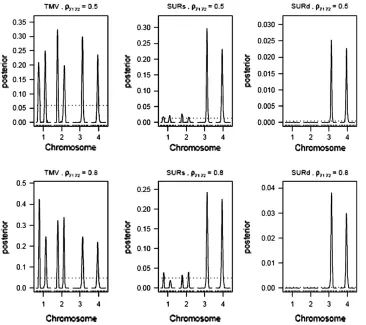
Figures 4–6 display the posterior probability profiles for the three sample sizes for testing pleiotropy (a certain locus is simultaneously included in the model for both traits) in the TMV, SURs, and SURd frame-works. We follow the same procedure to measure the

threshold values for pleiotropic posterior probabilities. As can be seen in Figure 4, TMV incorrectly detectedQ1 andQ3as pleiotropic QTL in the low correlation case; but in the high correlation case it could only feebly detect the true moderate pleiotropic QTL (Q5) in addition to the incorrectly detected ones; SURs de-tectedQ5 correctly andQ3 incorrectly in both correla-tion structures; SURd incorrectly detectedQ3in the low correlation case, but correctly detected both pleiotro-pic QTL (Q5 andQ6) in the high correlation case. In Figures 4 and 6, TMV incorrectly detected all 6 QTL as pleiotropic QTL in both correlation structures. In Figures 5 and 6, SURs detected both pleiotropic QTL correctly but also detected some extraneous nonpleio-tropic QTL for both correlation structures. SURd, how-ever, detected both pleiotropic QTL correctly without any incorrect detection in the small and large sample size situations for both correlation structures.

The average times taken to conduct each MCMC for all six cases and four methods are presented in Table 3. TMV was the fastest in all cases followed by SURs, STA, and SURd. However, the maximum difference between the fastest and the slowest was only 1.62 min (1 min 37 sec). So computationally complexity does not really pose a great threat.

In conclusion, it is evident and expected that the multivariate procedures outperform STA in the small sample size and high correlation situations. However, one should not use the traditional multivariate model Figure 5.—Profile of posterior

to detect nonpleiotropic QTL as there was astounding evidence of it being prone to erroneous detection. Both the SUR models performed well, but SURs provided slightly false evidence for a QTL influencing y1 (say) for y2. If one wants to detect only pleiotropic QTL, a traditional multivariate model can be used, but, in any other situations, a SURd procedure is recommended in light of a marginal increase in computational time.

DISCUSSION

Our goal in this article was to develop a comprehen-sive genomewide QTL mapping technique for multiple traits and assess its performance with existing single-trait analysis. When a QTL mapping experiment is con-ducted, an experimenter rarely measures only a single trait. However, even in the presence of data on more than one trait, there has been a lack of joint analysis of all traits primarily due to the lack of a comprehensive multivariate multiple-QTL mapping technique. From the simulation experiments we have observed that for relatively highly correlated traits the performance of multivariate methods is better compared to single-trait analysis in terms of QTL identification.

We have proposed two separate models for the joint analysis of multiple traits, namely, the seemingly un-related regression and the traditional multivariate model. The advantage of the SUR model is that it

per-mits all traits to have separate genetic models, much like an independent trait-by-trait analysis but including the correlation structure between the traits, thereby making it more powerful and precise. The traditional multivar-iate model, however, assumes the same genetic model for all traits. In the situation that we considered in the simulation experiment, we saw poor performance of the traditional multivariate model in terms of accuracy and extraneous detections. The traditional multivariate model is appropriate in the extreme sense when all detectable QTL are pleiotropic (influencing all traits simultaneously). Rarely, knowledge of this magnitude about a complex trait is knowna priori.In general, we recommend using a SUR model.

We investigated two different QTL SUR models, namely, SURs and SURd. The performance of both Figure6.—Profile of posterior

inclusion probabilities for the test of pleiotropy for n ¼ 500. The dotted line represents the 95% threshold for the null model. On thex-axis, large tick marks repre-sent chromosomes and small tick marks represent markers.

TABLE 3

Average MCMC time (in minutes) for four methods

ðn;r_y1y2Þ STA TMV SURs SURd

these QTL SUR models has been good. SURs can favor, though very slightly, a QTL of no effect on one trait but having large effect on another trait. In these situations SURd is recommended, since it consistently inferred the correct underlying genetic architecture in simula-tions. However, the current sampling scheme for updating the genotypes of pleiotropic QTL based on SURd may be suboptimal (as indicated by one of the reviewers), because we always treat the genotypes for different traits separately. In the case where inferring genotypes is difficult we would advocate the use of SURs or replace the genotypes by their conditional expecta-tion in our QTL SUR models (i.e., similar to Haley– Knott regression in QTL analysis). We also can improve the step of updating the genotypes of pleiotropic QTL by using a joint sampling method.

We have adopted the composite model space ap-proach (Yi 2004) and extended it to the multivariate case. The advantage of this approach is that it provides a very efficient way to walk through the space of models, spending more time at ‘‘good’’ models. The key idea behind this approach is to reduce a variable dimen-sional problem (number of unknown QTL) to a fixed dimensional space and impose a constraint on the maximum number of QTL that can be detected. Our MCMC algorithm has smart strategies to improve efficiency and conduct genomewide scans quickly. For example, we developed a novel one-at-a-time Gibbs sampler to sample regression coefficients that allows us to avoid inverting matrices, saving a lot of precious computational time. In high dimensional problems, in-verting extremely large matrices for typically.100,000 iterations can be very computationally taxing and prohibits the use of a multivariate algorithm (as seen in the implementation of Verzilliet al.2005). We also use the inverse of the variance–covariance matrix for the same reason. We have used informative hierarchical priors for the regression coefficients that typically re-flect most QTL mapping situations.

We have developed SUR models for QTL that act in a strictly additive manner. However, it is important to mention that this might not be a good assumption especially in light of the growing number of QTL studies providing evidence in favor of interactions between QTL. Our method can extend to include gene–gene and gene– environment interactions in a natural way. In the pres-ence of such interactions, the search space for possible QTL increases dramatically. We plan to investigate the performance of epistatic SUR methods in the future. We also plan to extend the multivariate framework to a mixture of continuous, binary, and ordinal traits.

We thank the reviewers for their helpful comments on the previous version of this manuscript. This work was supported by the following National Institutes of Health grants: R01 GM069430 (N.Y. and B.Y.), National Institute of Diabetes and Digestive and Kidney Diseases (NIDDK) 5803701 (B.Y.), NIDDK 66369-01 (B.Y.), and National Institute of General Medical Sciences/R01 PA-02-110 (B.Y.).

LITERATURE CITED

Ball_{, R. D., 2001 Bayesian methods for quantitative trait loci}

map-ping based on model selection: approximate analysis using the Bayesian information criterion. Genetics159:1351–1364. Broman, K. W., and T. Speed, 2002 A model selection approach for

the identification of quantitative trait loci in experimental crosses. J. R. Stat. Soc. B64(4): 641–656.

Broman_{, K. W., H. W}u_{, S´. S}en_{and G. A. C}hurchill_{, 2003 R/qtl:}

QTL mapping in experimental crosses. Bioinformatics 19:

889–890.

Burnham, K. P., and D. R. Anderson, 2002 Model Selection and

Multi-Model Inference.Springer-Verlag, New York.

Gelman_{, A., J. C}arlin_{, H. S}tern_{and D. R}ubin_{, 2004 Bayesian Data}

Analysis.Chapman & Hall/CRC, London.

Gilbert_{, H., and P. L}e_Roy_{, 2003 Comparison of three multitrait}

methods for QTL detection. Genet. Sel. Evol.35:281–304. Gilbert_{, H., and P. L}e_Roy_{, 2004 Power of three multitrait methods}

for QTL detection in crossbreed populations. Genet Sel. Evol.36:

347–361.

Griffiths, W. E., 2001 Bayesian Inference in the Seemingly Unrelated

Regressions Model (Working Series Paper 793). Department of Economics, University of Melbourne, Melbourne, Australia. Hackett, C. A., R. C. Meyerand W. T. B. Thomas, 2001 Multi-trait

QTL mapping in barley using multivariate regression. Genet.

Res. Camb.77:95–106.

Huang_{, J., and Y. J}iang_{, 2003 Genetic linkage analysis of a}

dichot-omous trait incorporating a tightly linked quantitative trait in af-fected sib pairs. Am. J. Hum. Genet.72:949–960.

Jackson, A. U., A. Forne´ s, A. Galecki, R. A. Millerand D. T. Burke,

1999 Multiple-trait quantitative trait loci analysis using a large

mouse sibship. Genetics151:785–795.

Jiang_{, C., and Z.-B. Z}eng_{, 1995 Multiple trait analysis of genetic}

mapping for quantitative trait loci. Genetics140:1111–1127. Jiang_{, C., and Z.-B. Z}eng_{, 1997 Mapping quantitative trait loci with}

dominant and missing markers in various crosses from two in-bred lines. Genetica101:47–58.

Kao, C.-H., and Z.-B. Zeng, 2002 Modeling epistasis of quantitative

trait loci using Cockerham’s model. Genetics160:1243–1261. Knott, S. A., and C. S. Haley, 2000 Multitrait least squares for

quantitative trait loci detection. Genetics156:899–911. Lander_{, E. S., and D. B}otstein_{, 1989 Mapping Mendelian factors}

underlying quantitative traits using RFLP linkage maps. Genetics

121:185–199.

Lange, C., and J. C. Whittaker, 2001 Mapping quantitative trait

loci using generalized estimating equations. Genetics159:1325– 1337.

Liu_{, J., Y. L}iu_{, X. L}iu_{and H.-W. D}eng_{, 2007 Bayesian mapping of}

quantitative trait loci for multiple complex traits with the use

of variance components. Am. J. Hum. Genet.81:304–320.

Lund, M. S., P. Sørensen, B. Guldbrandtsenand D. A. Sorensen,

2003 Multitrait fine mapping of quantitative trait loci using

combined linkage disequilibria and linkage analysis. Genetics

163:405–410.

Ma¨ hler, M., C. Most, S. Schmidtke, J. P. Sundberg, R. Liet al.,

2002 Genetics of colitis susceptibility in IL-10-deficient mice: backcross versus F2 results contrasted by principal component analysis. Genomics80:274–282.

Mangin_{, B., P. T}hoquet_{and N. G}rimsley_{, 1998 Pleiotropic QTL}

analysis. Biometrics54:88–99.

Meuwissen_{, T. H., and M. E. G}oddard_{, 2004 Mapping multiple}

QTL using linkage disequilibrium and linkage analysis informa-tion and multitrait data. Genet. Sel. Evol.36:261–279. Miller, A. J., 1984 Selection of subsets of regression variables. J. R.

Stat. Soc. A147:389–425.

Plummer, M., N. Best, K. Cowlesand K. Vines, 2004 Output

Anal-ysis and Diagnostics for MCMC, v. 0.9–5. Institute of Mathematical Statistics, Beachwood, OH.

Raftery, A. E., D. Madigan and J. A. Hoeting, 1997 Bayesian

model averaging for linear regression models. J. Am. Stat. Assoc.

92:179–191.

Satagopan_{, J. M., and B. S. Y}andell_{, 1996 Estimating the number}

Sen, S´., and G. A. Churchill, 2001 A statistical framework for

quan-titative trait mapping. Genetics159:371–387.

Sillanpa¨ a¨, M. J., and J. Corander, 2002 Model choice in gene

map-ping: what and why. Trends Genet.18:301–307.

Smith, M., and R. Kohn, 2000 Nonparametric seemingly unrelated

regression. J. Econometrics98:257–281.

Verzilli, C. J., N. Stallardand J. C. Whittaker, 2005 Bayesian

modeling of multivariate quantitative traits using seemingly un-related regression. Genetic Epidemiol.28:313–325.

Vieira, C., E. G. Pasyukova, Z.-B. Zeng, J. B. Hackett, R. F. Lyman

et al., 2000 Genotype-environment interaction for quantitative trait loci affecting life span in Drosophila melanogaster.Genetics

154:213–227.

Wang, H., Y. C. M. Zhang, X. Li, G. L. Masinde, S. Mohanet al.,

2005 Bayesian shrinkage estimation of quantitative trait loci

parameters. Genetics170:465–480.

Williams, J. T., H. Begleiter, B. Porjesz, H. J. Edenberg, T. Foroud

et al., 1999a Joint multipoint linkage analysis of multivariate qualitative and quantitative traits. II. Alcoholism and event-related potentials. Am. J. Hum. Genet.65:1148–1160. Williams, J. T., P. VanEerdewegh, L. Almasyand J. Blangero,

1999b Joint multipoint linkage analysis of multivariate qualita-tive and quantitaqualita-tive traits. I. Likelihood formulation and simu-lation results. Am. J. Hum. Genet.65:1134–1147.

Xu, C., Z. Liand S. Xu, 2005 Joint mapping of quantitative trait loci

for multiple binary characters. Genetics169:1045–1059. Yang, R., and S. Xu, 2007 Bayesian shrinkage analysis of quantitative

trait loci for dynamic traits. Genetics176:1169–1185.

Yandell, B. S., T. Mehta, S. Banerjee, D. Shriner, R. Venkataraman

et al., 2007 R/qtlbim: QTL with Bayesian interval mapping in experimental crosses. Bioinformatics23(5): 641–643.

Yi, N., 2004 A unified Markov chain Monte Carlo framework for

mapping multiple quantitative trait loci. Genetics167:967–975. Yi, N., and D. Shriner, 2008 Advances in Bayesian multiple QTL

mapping in experimental designs. Heredity100:240–252.

Yi, N., and S. Xu, 2002 Mapping quantitative trait loci with epistatic

effects. Genet. Res. Camb.79:185–198.

Yi, N., S. Xuand D. B. Allison, 2003 Bayesian model choice and

search strategies for mapping interacting quantitative trait loci.

Genetics165:867–883.

Yi_{, N., B. S. Y}andell_{, G. A. C}hurchill_{, D. B. A}llison_{, E. J. E}isen_{et al.,}

2005 Bayesian model selection for genomewide epistatic

quan-titative trait loci analysis. Genetics170:1333–1344.

Yi, N., D. Shriner, S. Banerjee, T. Mehta, D. Pomp_{et al.}, 2007 An

efficient Bayesian model selection approach for interacting QTL

models with many effects. Genetics176:1865–1877.

Zellner, A., 1962 An efficient method of estimating seemingly

un-related regressions and tests for aggregation bias. J. Am. Stat. Assoc.57:348–368.

Zeng_{, Z.-B., T. W}ang_{and W. Z}ou_{, 2005 Modeling quantitative trait}

loci and interpretation of models. Genetics169:1711–1725.

Communicating editor: J. B. Walsh

APPENDIX A: PRIOR DISTRIBUTIONS

The independent priors across traits are straightforward extensions of Yiet al. (2005, 2007). We describe the priors onðlt;gt;mt;btÞfor each trait, highlighting the distinctions pertinent to multiple correlated traits.

The prior distribution on QTL locations is uniformly distributed over the preset loci across the genome (Yiet al. 2005). Two constraints can be incorporated into the prior on QTL locations to reduce the model space: the first restricts the spacing among multiple linked QTL and the second restricts the number of detectable QTL on each chromosome (see Yiet al. 2007).

For the vector of indicatorsgt, we could use an independence prior,pðgtÞ ¼

Q

jw

g_tj

t ð1wtÞ1

gtj_{, withwtbeing the}

prior inclusion probability of each effect for thetth trait. A useful reduction can be achieved by settingw1 ¼ ¼wT. To specifywt, we first determine the prior expected numbers of main-effect QTL and then solve for wt from the expressions of the prior expected numbers (see Yiet al.2005). The prior expected number of main-effect QTL could be set to the number of QTL detected by traditional mapping methods.

The prior for the overall meanm_tis chosen to be normally distributed with mean and variance being sample mean and variance of thetth trait, respectively. For the genetic effectsb_t, we extend the prior of Yiet al. (2007) that assumes that different types of effects (e.g., additive effects or dominance effects) follow different prior distributions. For typek, effectsbk

tjhave the prior,b k

tjjgtj ð1gtjÞI01gtjNð0;s2tkÞ, wheregtjis the indicator variable forbktj, andI0is a point mass at 0. Under this prior, wheng_tj ¼0,bk

tj is assigned to be 0 and thus is actually removed from the model; when

g_kj ¼1,bk

tjfollows a normal distributionNð0;s

2

tkÞ. The variances

2

tkis treated as a random variable with an inverse-x 2

hyperprior distribution;i.e.,s2

tk Inv-x2ðntk;stk2Þ. The degrees of freedomntkcontrol the skewness of the prior fors2tk, with larger values recommended (herentk¼6) to tightly center the prior arounds2tk(see Yiet al. 2007). The scale parameters2

tkcontrols the prior proportion of phenotypic variance explained byb k

tj. We sets2tk¼ ðntk2ÞhVt=ðntkVtjkÞ, leading to the proportion of phenotypic variance explained bybk

tjbeingh, whereVtis the phenotypic variance of traitt, andVk

tj is the sample variance for the column ofXassociated with effectb k

tj. Expected effect heritability,h, can be set small (say 0.05–0.2) to reflect prior knowledge about genetic architecture.

APPENDIX B: CONDITIONAL POSTERIOR DISTRIBUTIONS

Conditional posterior distribution of eachmt:The conditional posterior distribution for the overall mean of thetth

trait,m_t, can be shown to be

m_tju;yN

Pn

i¼1ðyimtXibÞSt1

nS_tt1 ;

1 nS_tt1

!

; ðB1Þ

whereurepresents all elements ofuexceptmt,mtis the vectormwith thetth elementmtreplaced by 0,S

1

t is thetth column ofS1, andS_tttis the (t,t) element ofS1. Since the conditional posterior is a standard distribution, a Gibbs sampler can be easily performed.

Conditional posterior distribution of each btj: If thejth effect of thetth trait,btj, is included in the model, the conditional posterior distribution ofb_tjcan be shown to be

b_tjju;yN

Pn

i¼1xtijðyimXibtjÞSt1

S1

tt

Pn

i¼1x2tij1s

2

tj

; 1

S1

tt

Pn

i¼1xtij2 1s

2

tj

!

; ðB2Þ

whereurepresents all elements ofuexceptbtj,btjis the vectorbwith the elementbtjreplaced by 0,S

1

t andS

t tt are defined as in (A1), andxtijis the main-effect contrast for thejth effect for thetth trait and theith individual. Note that xtij¼xij"tfor SURs and TMV.

Conditional posterior distribution of each stk2: For each type of genetic effects (additive and dominance), the

conditional posterior distribution ofs2

tkis an inverse-x

2_{distribution,}

s2_tkju;y Inv-x2 ntk1qtk;

ntkstk2 1

P

jðbktjÞ2

n_tk1qtk

!

; ðB3Þ

whereqtkis the number of nonzero effects infbk

tj;j¼1;2; g, and other parameters are defined earlier.

Conditional posterior distribution ofS1_{:Keeping the computationally efficient goal in mind, it should be noted}

that generatingSwould involve computing its inverse to draw samples from (B1) and (B2) in each iteration. So, it is not only convenient to work withS1but computationally efficient as well. The conditional posterior distribution for S1can be calculated

S1ju;y jS1jð1=2ÞðnT1Þexp 1 2trðVS

1_Þ

¼WishartTðV1;nÞ; ðB4Þ

whereurepresents all elements ofuexceptS 1

, andVis aT3Tmatrix of residuals where the (t,t9)th element ofV,

vtt9¼Pn_i¼1

ytimˆ_tP_jbˆ_tijxtijyt9imˆt9

P

jbˆt9ijxt9ij

. Since the posterior of S1 follows a standard Wishart distribution, a Gibbs sampler can be used to generate samples. An alternative Metropolis algorithm could also be used to generate samples where a newly generated iterateS_new1 is accepted over an old valueS_old1 with probability

a¼min 1;pðS 1

newju;yÞqðS 1 oldÞ

pðS_old1ju;yÞqðSnew1 Þ

¼min 1;jS 1 newjn

=2_expfð1=2Þ

trðVS_old1Þg jS_old1jn=2_{expfð1=2ÞtrðVS}1

newÞg

( )

; ðB5Þ

whereq(.) is the proposal density that is assumed to be the same as its prior. We have implemented both the Gibbs sampler and the Metropolis algorithm for updatingS1and in either case we get similar results.

Conditional posterior distribution of eachgtiq:If locusqfor traittis included in the model and the genotypegtiqof

individualiis not observed, the conditional posterior distribution ofgtiq is

pðgtiq ¼kju;y_iÞ}pðy_iju;y_i;gtiq ¼kÞpðgtiq ¼kjltqÞ; ðB6Þ

whereurepresents all elements ofuexceptgtiq,pðy_iju;y_i;gtiq ¼kÞis the likelihood for individualicalculated by

model (2), andpðgtiq ¼kjl_qÞis the prior probability ofgtiq ¼k. This posterior is a simple multinomial distribution and thus can be sampled directly. If locusqis excluded from the model orgtiqis observed (e.g., for fully observed markers), we do not need to samplegtiq.

Conditional posterior distribution ofl:If locusqfor traittis included in the model, the joint conditional posterior distribution of the positionl_tqand the genotypesg_tq¼ ðgt1q; ;gtnqÞis

whereurepresents all elements ofuexceptltq andgtq,pðyju;ltq;g_tqÞis the likelihood calculated by model (2), pðltqÞis the prior ofltq, andpðg_tqjltqÞ ¼Qni¼1pðgtiqjltqÞis the prior probability ofgtq.

This posterior is not a standard distribution, and thus a Metropolis algorithm is needed to update ltq andgtq jointly. We first propose a new positionl*

tqfrom a proposal distributionqðl

*

tq;ltqÞand then generate new genotypes, g*

tiq, at this new position for all individuals from the conditional posterior (B6). The proposals forl

*

tqandg

*

tqare then accepted simultaneously with probability

a¼min 1;pðl *

tq;g

*

tqju;yÞqðltq;l*tqÞqðgtqÞ pðl_tq;g_tqju;yÞqðl*_tq;ltqÞqðg*tqÞ

!

: ðB8Þ

The proposal distribution for the new positionqðl*

q;lqÞis usually constructed as uniformly distributed over 2dmost flanking loci oflq, withdbeing a predetermined tuning integer. In our implementation, we taked¼2 and incorporate the preset constraints on QTL positions into our algorithm.

Conditional posterior distribution of each gtj:The conditional posterior distribution ofgtjcan be expressed as

pðg_tj¼1ju;yÞ ¼ pðgtj ¼1Þpðyju;gtj¼1Þ

pðg_tj ¼0Þpðyju;gtj ¼0Þ1pðgtj¼1Þpðyju;gtj¼1Þ

; ðB9Þ

whereurepresents all elements ofuexceptgtjandbtj,pðyju;gtj¼0Þis calculated using model (2) withbtjreplaced by 0, andpðyju;gtj ¼1Þdoes not depend onbtj and can be calculated using the identity of simple conditional probability

pðyju;gtj¼1Þ ¼

pðyju;g_tj¼1;b_tjÞpðb_tjÞ

pðb_tjjy;u;g_tj¼1Þ ; ðB10Þ

wherepðyju;gtj ¼1;btjÞis the phenotype likelihood calculated using model (2),pðbtjÞis the prior distribution ofbtj, andpðb_tjjy;u;gtj¼1Þis the conditional posterior distribution ofbtjcalculated by (B2). Notationally, the right side of (B10) depends onb_tj, but from the definition ofpðyju;gtj¼1Þ, we know it cannot depend onbtjin a real sense. That is, the factors that depend onb_tj in the numerator and the denominator must cancel. Thus, we can compute (B10) by inserting any value ofb_tjinto the expression. A convenient, stable choice is the conditional posterior mean of

b_tj(Gelmanet al.2004; Yiet al.2007).

To calculate the conditional posterior probability (B9), we may need the values of parameters associated withg_tj. If

g_tjis currently 0 and the involved QTL(s) is (are) not currently in the model, we first sample new QTL position(s) from their corresponding priors as needed, new genotypes for all individuals, and the prior variance ofb_tjif this parameter is currently out of the model. If the current value ofg_tjis 1, the associated unknowns were already generated at the preceding iteration.

The Gibbs sampler can be used to generate each indicatorg_tjfrom its conditional posterior (B9). However, for the QTL SUR models, using the Gibbs samplers is computationally demanding because the SUR models containTtimes the number of indicators as a single-trait model and most of the indicators are zero. To speed up the algorithm we extend the Metropolis–Hastings algorithm proposed by Yiet al. (2007) to the QTL SUR models. As with the Gibbs sampler, the MH scheme proceeds to update all indicator variables. Denote the current value ofg_tjbyC(¼0 or 1). The MH algorithm proposes a new valueP (¼0 or 1) for g_tj from the prior probabilityp(gtj¼C). IfP ¼C, the MH acceptance probability is 1, and thusgtjremains atCand there is no need to compute any values. Otherwise, we update

gtjfrom the current valueCto the proposal 1Cwith acceptance probability

a¼min 1;pðgtj¼1Cju;yÞ pðg_tj¼Cju;yÞ

pðgtj¼CÞ

pðg_tj¼1CÞ

!

; ðB11Þ

wherepðg_tj¼Cju;yÞandpðgtj ¼1Cju;yÞare calculated in (B9).

The conditional posterior ofgfor the traditional multivariate model is a little tricky. Since the indicator variable of a particular effect is the same for all traits, the conditional posterior distribution ofg_j can be expressed as

pðg_j ¼1ju;yÞ ¼

pðg_j¼1Þpðyju;gj ¼1Þ

pðg_j¼0Þpðyju;gj¼0Þ1pðgj ¼1Þpðyju;gj¼1Þ

; ðB12Þ

whereg_j is the indicator variable for thejth effects for all traits,urepresents all elements ofuexceptgj andb ˜j,

b

˜j denotes the vector of thejth effects for all traits, andpðyju;gtj ¼0Þis calculated using model (2) withb

0. The integration in (B10) should be with respect to joint distribution of all genetic effects for the traits in question. Proceeding similarly as above we can get

pðyju;gj ¼1Þ ¼

pðyju;gj ¼1;b

˜j

Þpðb

˜j

Þ

pðb

˜j

jy;u;gj ¼1Þ

: ðB13Þ

As before, a choice ofb

˜j could be the posterior mean of the joint posterior distribution of

b

˜j calculated below,

b

˜jNT

Sb

Xn

i¼1

xijS1ðyimx9ib ˜jÞ

;Sb

!

; ðB14Þ

wherexi is the vector of main-effect contrast(s) for theith individual for all loci,Sb¼

S1Pn_i¼1x2

ij1diagðs ˜

2

j Þ

1

,

s

˜ 2

j is the vector of the variances of thejth genetic effect for all traits, andb ˜

jis the vector of coefficients withbtj(t¼1,