Towards a redundancy elimination algorithm
for underspecified descriptions
Alexander Koller and Stefan Thater
Department of Computational Linguistics Universität des Saarlandes, Saarbrücken, Germany
{koller,stth}@coli.uni-sb.de
Abstract
This paper proposes an efficient algorithm for theredundancy eliminationproblem: Given an underspecified semantic representation (USR), compute an USR which has fewer read-ings, but still describes at least one representative of each semantic equivalence class of the original readings. The algorithm operates on underspecified chart representations which are derived from dominance graphs; it can be applied to the USRs computed by large-scale grammars. To our knowledge, it is the first redundancy elimination algorithm which maintains underspecification, rather than just enumerating non-redundant readings.
1
Introduction
Underspecification is the standard approach to dealing with scope ambiguities in computational semantics [12,6,7,2]. The basic idea is to not enumerate all possible semantic representations for each syntactic analysis, but to derive a single compact underspecified representation (USR). This simplifies semantics construction, and current algorithms support the efficient enumeration of readings from an USR [10].
In addition, underspecification has the potential for eliminating incorrect or re-dundant readings by inferences based on context or world knowledge, without even enumerating them. For instance, sentences with scope ambiguities often have read-ings which are semantically equivalent. In this case, we typically need to retain only one reading from each equivalence class. This situation is illustrated by the following two sentences from the Rondane treebank, which is distributed with the English Resource Grammar (ERG; [5]), a broad-coverage HPSG grammar.
(1) For travellers going to Finnmark there is a bus service from Oslo to Alta
through Sweden. (Rondane 1262)
(2) We quickly put up the tents in the lee of a small hillside and cook for the first
time in the open. (Rondane 892)
phrases (including proper names and pronouns). The USR for (1) describes 3960 readings, which are all semantically equivalent to each other. On the other hand, the USR for (2) has 480 readings, which fall into two classes of mutually equivalent readings, characterised by the relative scope of “the lee of” and “a small hillside.”
This paper presents an algorithm for theredundancy eliminationproblem: Given
an USR, compute an USR which has fewer readings, but still describes at least one representative of each equivalence class – without enumerating any readings. This algorithm computes the one or two representatives of the semantic equivalence classes in the above examples, so subsequent modules don’t have to deal with all the other equivalent readings. It also closes the gap between the large number of readings predicted by the grammar and the intuitively perceived much lower degree of ambiguity of these sentences. Finally, it can be helpful for a grammar designer because it is much more feasible to check whether two readings are linguistically reasonable than 480.
We model equivalence in terms of rewrite rules that permute quantifiers without changing the semantics of the readings. The particular USRs we work with are un-derspecified chart representations, which can be computed from dominance graphs (or USRs in some other underspecification formalisms) efficiently [10]. The algo-rithm can deal with many interesting cases, but is incomplete in the sense that the resulting USR may still describe multiple equivalent readings.
To our knowledge, this is the first algorithm in the literature for redundancy
elimination on the level of USRs. There has been previous research onenumerating
only some representatives of each equivalence class [13,4], but these approaches don’t maintain underspecification: After running their algorithms, we have a set of readings rather than an underspecified representation.
Plan of the paper. We will first define dominance graphs and review the necessary background theory in Section 2. We will then give a formal definition of equiva-lence and derive some first results in Section 3. Section 4 presents the redundancy elimination algorithm. Finally, Section 5 concludes and points to further work.
2
Dominance Graphs
The basic underspecification formalism we assume here are labelled dominance
graphs [1]. Dominance graphs are equivalent to leaf-labelled normal dominance constraints [7], which have been discussed extensively in previous literature.
Definition 2.1 A(compact) dominance graph is a directed graph(V,E]D)with
two kinds of edges,tree edges E anddominance edges D, such that:
(i) the graph(V,E)defines a collection of node disjoint trees of height 0 or 1. We call the trees in(V,E)thefragmentsof the graph.
(ii) if(v,v0)is a dominance edge inD, thenvis a hole andv0is a root inG. A node vis aroot(inG) ifvdoes not have incoming tree edges; otherwise,vis ahole.
ay sampley seex,y ax repr-ofx,z az compz
1 2 3
4 5 6
7 ay ax az 1 2 3
sampley seex,y repr-ofx,z
compz
ay
ax
sampley seex,y
[image:3.595.109.497.76.147.2]repr-ofx,z az compz 1 2 3
Fig. 1. A dominance graph that represents the five readings of the sentence “a representative of a company saw a sample” (left) and two (of five) configurations.
1 2 3
4 5 6
7 h2
h1 h3 h4 h5 h6
1 3
4 5 6
7 h2
h1 h5 h6
→ → h2 h1 h4 h3 h6 h5 2 1 3
4 5 6 7
Fig. 2. An example computation of a solved form.
such that (V,E]D) is a dominance graph and L:V Σ is a partial labelling
functionwhich assigns a nodeva label with arityniff vis a root withnoutgoing tree edges. Nodes without labels (i.e., holes) must have outgoing dominance edges.
We will writev:f(v1, . . . ,vk)for a fragment whose rootvis labelled with f and
whose holes arev1, . . . ,vk. We will writeR(F)for the root of the fragmentF, and
we will typically just saygraphinstead oflabelled dominance graph.
An example of a labelled dominance graph is shown to the left of Fig. 1. Tree edges are drawn as solid lines, and dominance edges are drawn as dotted lines, di-rected from top to bottom. This graph can serve as an USR for the sentence “a repre-sentative of a company saw a sample” if we demand that the holes are “plugged” by
roots while realising the dominance edges as dominance, as in the two (of five)
con-figurations shown to the right [7]. Configurations encode semantic representations
of the sentence, and we freely read configurations as ground terms overΣ.
2.1 Solving dominance graphs
Algorithms forsolving a dominance graph in order to compute the readings it
de-scribes typically compute itsminimal solved forms[1,3]. In this paper, we restrict
ourselves to hypernormally connected graphs (defined below), for which one can
show that all solved forms are minimal and bijectively correspond to configurations.
LetG,G0be dominance graphs. We say thatGisin solved formiff it is a forest,
andGis asolved form of G0ifGis in solved form and more specific thanG0i.e.,G
andG0 have the same labels and tree fragments, and the reachability relation ofG
extends that ofG0. G0issolvableif it has a solved formG. IfG0 is hypernormally
connected, then each hole in Ghas exactly one outgoing dominance edge, and G
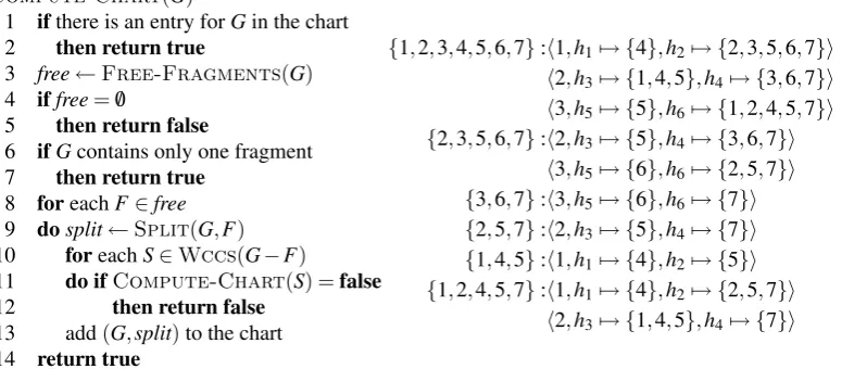
[image:3.595.133.474.198.273.2]Compute-Chart(G)
1 ifthere is an entry forGin the chart
2 then return true
3 free←Free-Fragments(G)
4 iffree=0/
5 then return false
6 ifGcontains only one fragment
7 then return true
8 foreachF∈free
9 dosplit←Split(G,F)
10 foreachS∈Wccs(G−F)
11 do ifCompute-Chart(S) =false
12 then return false
13 add(G,split)to the chart 14 return true
{1,2,3,4,5,6,7}:h1,h17→ {4},h27→ {2,3,5,6,7}i
h2,h37→ {1,4,5},h47→ {3,6,7}i
h3,h57→ {5},h67→ {1,2,4,5,7}i
{2,3,5,6,7}:h2,h37→ {5},h47→ {3,6,7}i
h3,h57→ {6},h67→ {2,5,7}i
{3,6,7}:h3,h57→ {6},h67→ {7}i
{2,5,7}:h2,h37→ {5},h47→ {7}i
{1,4,5}:h1,h17→ {4},h27→ {5}i
{1,2,4,5,7}:h1,h17→ {4},h27→ {2,5,7}i
[image:4.595.113.501.81.251.2]h2,h37→ {1,4,5},h47→ {7}i
Fig. 3. The chart solver and an example chart computed for the dominance graph in Fig. 2.
The key concept of the solver we build upon is that of afree fragment [3]. A
fragmentF in a solvable graphGis free iff there is a solved form in whichF is at
the root. It can be shown that a fragment is free iff it has no incoming dominance edges and its holes are in different biconnected components of the graph i.e., they are disconnected if the root of the fragment is removed from the graph [3]. Remov-ing a free fragment from a graph splits the graph into different weakly connected
components (wccs) – one for each hole. Thus each free fragmentF induces asplit
ofG, which consists of a reference toF and a mapping of the other fragments to the hole to which they are connected. For instance, the example graph has three free fragments: 1, 2, and 3. By removing fragment 2, the graph is decomposed into two
wccs, which are connected to the holesh3andh4, respectively (see Fig. 2).
The solver [10] is shown in Fig. 3. It computes a chart-like data structure which assigns sets of splits to subgraphs. For each subgraph it is called on, the solver computes the free fragments, the splits they induce, and calls itself recursively on the wccs of each split. It records subgraphs and splits in the chart, and will not repeat work for a subgraph it has encountered before. The algorithm returns true iff the original graph was solvable. The chart tells us how to build the minimal solved forms of the graph: For each subgraphs, pick any split, compute a solved form for each wcc recursively, and plug them into the given hole of the split’s root fragment. As an example, the chart for the graph in Fig. 1 is shown to the right of Fig. 3.
Notice that the chart which the solver computes, while possibly exponentially larger than the original graph, is still exponentially smaller than the entire set of
readings because common subgraphs (such as {2,5,7} in the example) are
repre-sented only once. Thus the chart can still serve as an underspecified representation.
2.2 Hypernormally connected dominance graphs
hypernormal path in G. Hnc graphs are equivalent tochain-connected dominance
constraints [9], and are closely related to dominance nets[11]. The results in this
paper are restricted to hnc graphs, but this does not limit the applicability of our results: an empirical study suggests that all dominance graphs that are generated by current large-scale grammars are (or should be) hnc [8].
The key property of hnc dominance graphs is that their solved forms correspond to configurations, and we will freely switch between solved forms and their corre-sponding configurations. Another important property of hnc graphs which we will use extensively in the proofs below is that it is possible to predict which holes of fragments can dominate other fragments in a solved form.
Lemma 2.2 Let G be a hnc graph with free fragment F. Then all weakly connected components of G−F are hnc.
Proposition 2.3 Let F1,F2be fragments in a hnc dominance graph G. If there is a solved form S of G in which R(F1)dominates R(F2), then there is exactly one hole
h of F1 which is connected to R(F2) by a simple hypernormal path which doesn’t use R(F1). In particular, h dominates R(F2)in S.
Proof. Let’s say that F1 dominates F2 in some solved form S. There is a run of
the solver which computes S. This run chooses F1 as a free fragment before it
choosesF2. Let’s call the subgraph in which the split forF1is chosen,G0.G0is hnc
(Lemma 2.2), so in particular there is a simple hypernormal path from the holeh
ofF1 which is in the same wcc asF2 toR(F2); this path doesn’t useR(F1). On the
other hand, assume there were another holeh0ofF1which is connected toR(F2)by
a path that doesn’t useR(F1). Then the path viaR(F2)would connecthandh0even
ifR(F1)were removed, soh andh0would be in the same biconnected component
ofG, in contradiction to the assumption thatF1is free inG0.
For the second result, note thatF2is assigned to the holehin the split forF1.2
The following definition captures the complex condition in Prop. 2.3:
Definition 2.4 Let G be a hnc dominance graph. A fragment F1 in G is called a possible dominatorof another fragmentF2inGiff it has exactly one holehwhich
is connected toR(F2)by a simple hypernormal path which doesn’t useR(F1). We
writech(F1,F2)for this uniqueh.
3
Equivalence
can therefore approximate equivalence by using arewrite systemthat permutes frag-ments and defining equivalence of configurations as mutual rewritability as usual.
By way of example, consider again the two (equivalent) configurations shown in Fig. 1. We can obtain the second configuration from the first one by applying the following rewrite rule, which rotates the nodes 1 and 2:
ax(az(P,Q),R)→az(P,ax(Q,R)) (3)
The formulas on both sides of the arrow are semantically equivalent in first-order
logic for any choice of the subformulas P, Q, andR. Thus the equivalence of the
two configurations with respect to our one-rule rewrite system implies that they are also semantically equivalent.
While we will require that the rewriting approximation issound i.e., rewrites
formulas into equivalent formulas, we cannot usually hope to achievecompleteness
i.e., there will be semantic equivalences that are not modelled by the rewriting equivalence. However, we believe that the rewriting-based system will still prove to be useful in practical applications, as the permutation of quantifiers is exactly the kind of variability that an underspecified description allows.
We formalise this rewriting-based notion of equivalence as follows. The defini-tion uses the abbreviadefini-tionx[1,k) forx1, . . . ,xk−1, andx(k,n]forxk+1, . . . ,xn.
Definition 3.1 Apermutation system Ris a system of rewrite rules over a signature
Σof the following form:
f1(x[1,i),f2(y[1,k),z,y(k,m]),x(i,n]) → f2(y[1,k),f1(x[1,i),z,x(i,n]),y(k,m])
Thepermutability relation P(R)is the binary relationP(R)⊆(Σ×N)2which
con-tains exactly the pairs((f1,i),(f2,k))and((f2,k),(f1,i))for each such rewrite rule.
As usual, we say that two terms areequivalentwith respect toR,s≈Rt, iff there
is a sequence of rewrite steps and inverse rewrite steps that rewritesintot. We say
thatRissoundwith respect to a semantic notion of equivalence≡if≈R⊆ ≡. IfG
is a graph over ΣandRa permutation system, then we writeSCR(G)for the set of
equivalence classes Conf(G)/≈R, where Conf(G)is the set of configurations ofG.
A rewrite system (let’s call itRfol) which is sound for the standard equivalence
relation of first-order logic could use rule (3) and the three other permutations of two existential quantifiers, plus the following rule for universal quantifiers:
everyx(X,everyy(Y,Z))→everyy(Y,everyx(X,Z))
The other three permutations of universal quantifiers, as well as the permutations of universal and existential quantifiers, are not sound.
It is possible to computeSCR(G)by solvingGand using a theorem prover for
xi+1 xn
x1 xi-1 y1 yk-1 yk+1 ym
y1 yk-1 z yk+1 ym
F2 F1
… …
… vk …
v = ui
u
F2
F1
x1 xi-1 xi+1 xn
… …
… …
z v
ui
vk = u (a)
F2
W
F1 ui
?
vj vk
w
πr
πu
[image:7.595.112.498.74.160.2]v (b)
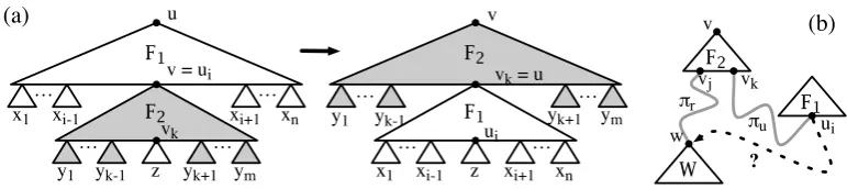
Fig. 4. Diagrams for the proof of Lemma 3.3
which hole of one fragment the other fragment can plug, we can’t know whether the
two fragments can be permuted. However, in ahnc graph, the hole of a fragment
which another fragment can plug is determined uniquely (because of Lemma 2.3), and can be recognised without solving the graph.
Definition 3.2 LetRbe a permutation system. Two fragmentsF1andF2with root
labels f1and f2in a graphGare calledR-permutableiff they are possible
domina-tors of each other and((f1,ch(F1,F2)),(f2,ch(F2,F1)))∈P(R).
Lemma 3.3 Let R be a permutation system, let F1 = u:f1(u1, . . . ,un) and F2 =
v:f2(v1, . . . ,vm)be R-permutable fragments in the hnc graph G, such that F2is free, and let C1be a configuration of G in which u is the father of v. Then:
(a) It is possible to apply a R-rewrite step or an inverse R-rewrite step to C1 at u; call the resulting tree C2.
(b) C2is also a configuration of G.
(c) C2≈RC1.
Proof. Leti=ch(F1,F2)andk=ch(F2,F1); we know that((f1,i),(f2,k))∈P(R). (a)F1is a possible dominator ofF2, souiis plugged withvinC1(Lemma 2.3).
Thus the (possibly inverse) rule which justified the tuple((f1,i),(f2,k))is applica-ble atu.
(b) We must verify that every dominance edge inGis realised byC2. As Fig. 4a
shows, all dominance edges that do not go out of a hole of F1 are still trivially
realised byC2. Now let’s consider dominances out of the holes ofF1.
• Dominance edges out of anyujwith j6=iare still satisfied (see the figure).
• Dominance edges fromuito a node inzare still satisfied (see the figure).
• Dominance edges fromuitov: Such edges cannot exist inGasF2is free.
• Dominance edges fromuito a nodewin someyj with j6=k: Such edges cannot
exist either. F2 is a possible dominator of the fragmentW whose root w is, so
there is a simple hypernormal pathπw fromch(F2,W)towwhich doesn’t usev;
ch(F2,W) =vj becausevj dominateswinC1 (Lemma 2.3). On the other hand,
F2 is a possible dominator ofF1, so there is a simple hypernormal pathπufrom
vk toui which doesn’t usev. Now if there were a dominance edge fromui tow
inG, thenvj and vk would be in the same biconnected component (they would be connected via πu◦(ui,w)◦π−w1 if v were removed), which contradicts the
4
Underspecified redundancy elimination
Now we can finally consider the problem of strengthening an USR in order to remove redundant readings which are equivalent to other readings. We will define
an algorithm which gets as its input a graphG, a chart as computed by COMPUTE
-CHART, and a permutability relationP(R). It will then remove splits from the chart,
to the effect that the chart represents fewer solved forms of the original graph, but at
least one representative from each class inSCR(G)remains. The subgraph sharing
of the original chart will be retained, so the computed chart is still an USR.
The key concept in the redundancy elimination algorithm is that of apermutable
split. Intuitively, a split of G is called permutable if its root fragment F is
per-mutable with all other fragments in G which could end up above F. Because of
Lemma 3.3, we can then always pull F to the root by a sequence of rewrite steps.
This means that for any configuration of G, there is an equivalent configuration
whose root isF – i.e., by choosing the split forF, we lose no equivalence classes.
Definition 4.1 LetR be a permutation system. A splitS of a graphG is called R-permutableiff the root fragmentF ofSisR-permutable with all other fragments in
Gwhich are possible dominators ofF inG.
In the graph of Fig. 1, all three splits areRfol-permutable: For each of the upper fragments, the other two upper fragments are possible dominators, but as all three
fragments are labelled with existential quantifiers andRfolcontains all permutations
of existential quantifiers, the fragments are permutable with each other. And indeed, we can pick any of the three fragments as the root fragment, and the resulting split will describe a representative of the single equivalence class of the graph.
Proposition 4.2 Let G be a hnc graph, and let S be a permutable split of G. Then SC(S) =SC(G).
Proof. If G is unsolvable, the claim is trivially true. Otherwise, letC be an arbi-trary configuration of G; we must show that S= (F,h17→G1, . . . ,hn7→Gn)has a
configurationC0which is equivalent toC.
Let’s say that the fragments which properly dominate F in C are F1, . . . ,Fn
(n≥0), ordered in such a way that Fi dominatesFj inC for alli< j. Each Fi is
a possible dominator ofF, by Prop. 2.3. BecauseSis permutable, this means that
eachFiis permutable withF inG. By applying Lemma 3.3ntimes (first toF and
Fn, then to F and Fn−1, and so on), we can compute a configurationC0 of G in
whichF is at the root and such thatC0≈RC. ButC is a configuration ofS, which
proves the theorem. 2
This suggests the following redundancy elimination algorithm:
Redundancy-Elimination(Ch,G,R)
1 foreach subgraphG0inCh
2 do ifG0has anR-permutable splitS
Because of Prop. 4.2, the algorithm is correct in that for each configurationCof G, the reduced chart still has a configurationC0withC≈RC0. The particular choice
of S doesn’t affect the correctness of the algorithm (but may change the number
of remaining configurations). However, the algorithm is not complete in the sense that the reduced chart can have no two equivalent configurations. We will illustrate this below. We can further optimize the algorithm by deleting subgraphs (and their splits) that are not referenced anymore by using reference counters. This doesn’t change the set of solved forms of the chart, but may further reduce the chart size.
In the running example, we would run REDUNDANCY-ELIMINATION on the
chart in Fig. 3. As we have seen, all three splits of the entire graph are permutable, so we can pick any of them e.g., the split with root fragment 2, and delete the splits with root fragments 1 and 3. This reduces the reference count of some subgraphs (e.g.{2,3,5,6,7}) to 0, so we can remove these subgraphs too. The resulting chart is shown below, which represents a single solved form (the one shown in Fig. 2).
{1,2,3,4,5,6,7}:h2,h27→ {1,4},h47→ {3,6,7}i
{1,4}:h1,h17→ {4}i
{3,6,7}:h3,h57→ {6},h67→ {7}i
Now consider variations of the graph in Fig. 1 in which the quantifier labels are different; these variant graphs have exactly the same chart, but fewer fragment pairs will be permutable. If all three quantifiers are universal, then the configurations fall into two equivalence classes which are distinguished by the relative scope of the fragments 1 and 2. The algorithm will recognise that the split with root fragment 3 is permutable and delete the splits for 1 and 2. The resulting chart has two solved forms. Thus the algorithm is still complete in this case. If, however, the fragments 1 and 2 are existential quantifiers and the fragment 3 is universal, there are three equivalence classes, but the chart computed by the algorithm will have four solved forms. The problem stems from the fact that neither of the existential quantifiers is permutable as long as the universal quantifier is still in the same subgraph; but the two configurations in which 2 dominates 3 are equivalent.
Runtime analysis. Given a graph Gwithnnodes andm edges, we can compute a
table which specifies for each pairu,vof root nodes whether there is a unique hole
ofufrom whichvcan be reached via a simple hypernormal path which doesn’t use
u, and which hole this is. A naive algorithm for doing this iterates over alluandv
and then performs a depth-first search through G, which takes time O(n2(n+m)),
which is a negligible runtime in practice.
Given this table, we can determine the possible dominators of each fragment
in time O(n) (because there are at most O(n) possible dominators). Thus it takes
5
Conclusion
We have presented an algorithm for redundancy elimination on underspecified chart
representations. It checks for each subgraph in the chart whether it has apermutable
split; if yes, it removes all other splits for this subgraph. This reduces the set of described readings, while making sure that at least one representative of each orig-inal equivalence class remains while maintaining underspecification. Equivalence is defined with respect to a certain class of rewriting systems which approximates semantic equivalence of the described formulas and fits well with the underspecifi-cation setting. The algorithm runs in polynomial time in the size of the chart.
The algorithm is useful in practice: it reduces the USRs for (1) and (2) from the introduction to one and two solved forms, respectively. In fact, initial experiments with the Rondane treebank suggest that it reduces the number of readings of a typical sentence by an order of magnitude. It does this efficiently: Even on USRs with billions of readings, for which the enumeration of readings would take about a year, it finishes after a few seconds. However, the algorithm is not complete in the sense that the computed chart has no more equivalent readings. We have some ideas for achieving this kind of completeness, which we will explore in future work. Another line in which the present work could be extended is to allow equivalence with respect to arbitrary rewrite systems.
References
[1] Althaus, E., D. Duchier, A. Koller, K. Mehlhorn, J. Niehren and S. Thiel,An efficient graph algorithm for dominance constraints, Journal of Algorithms48(2003), pp. 194–219.
[2] Blackburn, P. and J. Bos, “Representation and Inference for Natural Language. A First Course in Computational Semantics,” CSLI Publications, 2005.
[3] Bodirsky, M., D. Duchier, J. Niehren and S. Miele,An efficient algorithm for weakly normal dominance constraints, in:ACM-SIAM Symposium on Discrete Algorithms(2004).
[4] Chaves, R. P., Non-redundant scope disambiguation in underspecified semantics, in:
Proceedings of the 8th ESSLLI Student Session, Vienna, 2003, pp. 47–58.
[5] Copestake, A. and D. Flickinger, An open-source grammar development environment and broad-coverage english grammar using HPSG, in:Proc. of LREC, 2000.
[6] Copestake, A., D. Flickinger, C. Pollard and I. Sag, Minimal recursion semantics: An introduction., Journal of Language and Computation (2004), to appear.
[7] Egg, M., A. Koller and J. Niehren,The Constraint Language for Lambda Structures, Logic, Language, and Information10(2001), pp. 457–485.
[8] Fuchss, R., A. Koller, J. Niehren and S. Thater,Minimal recursion semantics as dominance constraints: Translation, evaluation, and analysis, in:Proc. of ACL, Barcelona, 2004.
[9] Koller, A., J. Niehren and S. Thater,Bridging the gap between underspecification formalisms: Hole semantics as dominance constraints, in:Proc. of EACL-03, 2003.
[10] Koller, A. and S. Thater,The evolution of dominance constraint solvers, in:Proc. of ACL-05 Workshop on Software, Ann Arbor, 2005.
[11] Niehren, J. and S. Thater,Bridging the gap between underspecification formalisms: Minimal recursion semantics as dominance constraints, in:Proc. of ACL-03, 2003.
[12] van Deemter, K. and S. Peters, “Semantic Ambiguity and Underspecification,” CSLI, 1996. [13] Vestre, E.,An algorithm for generating non-redundant quantifier scopings, in:Proc. of EACL,