Copyright2001 by the Genetics Society of America
Two-Generation Analysis of Pollen Flow Across a Landscape. II. Relation
Between
⌽
ft, Pollen Dispersal and Interfemale Distance
Fre´de´ric Austerlitz*
,†and Peter E. Smouse*
*Department of Ecology, Evolution and Natural Resources, Cook College, Rutgers University, New Brunswick, New Jersey 08901-8551 and †Laboratoire Evolution et Syste´matique, CNRS UPRESA 8079, Universite´ Paris-Sud, F-91405 Orsay Cedex, France
Manuscript received May 10, 2000 Accepted for publication November 10, 2000
ABSTRACT
We study the behavior of ⌽ft, a recently introduced estimator of instantaneous pollen flow, which is
basically the intraclass correlation of inferred pollen cloud genetic frequencies among a sample of females drawn from a single population. Using standard theories of identity by descent and spatial processes, we show that⌽ftdepends on the average distance of pollen dispersal (␦) and on the average distance between
sampled mothers (x1). Provided that mothers are sampled far enough apart (x1 ⬎ 5␦), ⌽ft becomes
independent ofx1and is then inversely proportional to the square of␦. Provided that this condition is fulfilled,␦is directly estimable from⌽ft. Even whenx1⬍5␦, estimation can easily be achieved via numerical
evaluation. We show that the relation between⌽ftand ␦is only modestly affected by the shape of the
distribution function, a result of importance, since this shape is generally unknown. We also study the impact of adult density within the population on⌽ft, showing that to achieve the correct inference of␦
from⌽ftit must be taken into account, but that it has no effect on the distance at which mothers must
be sampled.
M
OST authors (e.g., Slatkin and Barton 1989; tion distance across a landscape, sometimes a serious underestimate. Clearly, the estimation of real-time pol-Nath and Griffiths 1996; Beerli andFel-len dispersal must be addressed by some other means. senstein1999) have focused on the estimation of the
Smouseet al.(2001) have proposed a new estimation “historical” migration rate,i.e., the effective long-term
procedure, which uses only the genotypes of the moth-average (Hudson 1998). Such estimates are useful in
ers and of seedlings derived from them, along with the understanding the evolutionary history of a set of
popu-spatial positions of the mothers; the potentially contrib-lations, but they say nothing about the current level of
uting males are ignored. Using the sampled mothers as gene flow, a more relevant predictor of contemporaneous
strata and their seedlings as replicates, one estimates (real-time) genetic exchange among a set of populations.
the intraclass correlation of paternal gametes drawn from The need to estimate “real-time” gene flow rates has
a single mother,⌽ft, which is then used to estimate average led to the design of direct estimators of gene flow.
pollination distance. Based on a simulation study, The most used method is currently paternity analysis
Smouse et al. (2001) have shown that ⌽ft is directly (SchnabelandHamrick1995), which is especially
ef-related to the decay parameter of the pollen dispersal ficient when highly polymorphic markers are used
curve. (DowandAshley1996;Streiffet al.1999), but
conclu-The aim of this article is to address several questions sive analysis requires knowledge of the identity and
ge-that have been raised by ge-that first study: notypes of all potential males who could have
contrib-uted pollen to females within the stand. 1. How is⌽
ftaffected by the chosen dispersal function? Several studies (DowandAshley1996;Streiffet al. It will be difficult to derive a valid estimate of the
1999) have now shown that a substantial portion of average pollen dispersion from an estimate of⌽ftif pollen comes from outside the stand, and it has become that parameter is overly sensitive to the shape of the clear that characterizing all potential fathers that might (usually unknown) distribution.
have contributed pollen to the mothers within the stand 2. For any particular pollen dispersal distribution, what is virtually a hopeless task. Lacking the ability to identify is the precise relation between⌽ftand the dispersal and/or evaluate the external males, paternity analysis rate?
can provide only a minimum estimate of average pollina- 3. How is the estimate of ⌽ft affected by the average physical distance from one sampled mother to an-other?
4. What is the impact of adult density within the
refer-Corresponding author:Fre´de´ric Austerlitz, Laboratoire de Ge´ne´tique
et d’Ame´lioration des Arbres Forestiers, INRA—Domaine de l’Hermi- ence population? tage, B. P. 45, Pierroton, F-33611 Cestas Cedex, France.
E-mail: [email protected] Answers to these questions should allow us to design a
proper estimate of the average pollination distance from
⌽ft. We develop the theoretical framework necessary to address these issues.
THE MODEL
General context:Assume that we have an infinite pop-ulation, with adult individuals randomly distributed across the landscape, at density (d) per squared unit of distance. All individuals are monoecious and self-fertile, but they practice no more self-reproduction than would be expected at random. Allele frequencies are uniform across the landscape, all individuals are noninbred, and all have the same male fecundity. We assume that male gametes disperse independently and according to a probability distribution, to which we return below. We consider a sample of mothers drawn from among the adults, spaced an average distance ofx1apart. Mothers are chosen on the basis of spatial locations, but not on the basis of their genotypes. We assume that spatial positions and genotypes of adults are not correlated.
The genetic diversity within and among the pollen clouds impinging upon the various mothers depends upon the pollen dispersal distribution. We focus here on two isotropic two-dimensional distributions of pollen dispersal: the normal distribution and the exponential distribution. In Cartesian coordinates measured from a single mother, assumed to be at coordinates (0, 0), the normal distribution with parameterwill be
p(x,y)⫽ 1 22e
⫺(x2⫹y2)/22, (1)
where p(x, y) is the probability (or more precisely the
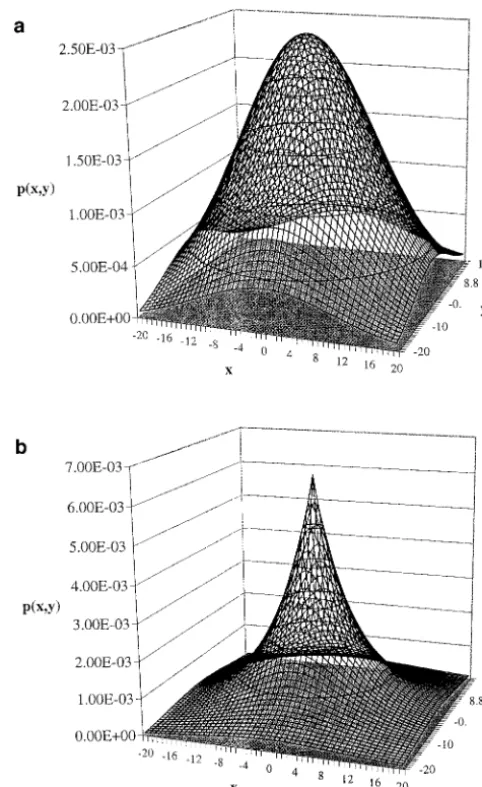
probability density function) that a single pollen grain Figure 1.—Probability density function p(x, y) plotted will have been drawn from coordinates (x,y). We define against the Cartesian coordinates (x,y), for the normal distri-bution (a) and the exponential distridistri-bution (b), for the same a corresponding exponential distribution, with
parame-value of the average dispersal distance␦ ⫽10. ter␥, as
p(x,y)⫽ 1 2␥2e
⫺√x2⫹y2/␥
. (2)
for both normal and exponential distributions, with the same average pollen dispersal distance,␦ ⫽ 10. These Both have mean positions of (0, 0) in Cartesian
coordi-curves have very different shapes; the exponential distri-nates, centered at the focal mother herself, and decline
bution has a sharp peak at zero, but it also has a greater monotonically (and isotropically) in every direction.
probability of reaching large dispersal distances. The average radial distance (␦) of pollen flow is
calcu-The different shapes of the two distributions affect lated as the expected value ofz, the average intermate
the dispersion of pollen distances for a given value of distance:
␦. One can gauge this dispersion via the variance of
␦ ⫽
冮
⫺∞∞
冮
∞ ⫺∞√
x2⫹y2p(x,y)dxdy. (3)
pollen dispersion, defined asv2⫽E(z2)⫺E2(z), where
z⫽(x2⫹y2)1/2is the linear distance from the position of the pollinating male (x, y) to the index female (0, For the normal distribution, that yields
0). Alternatively, one could use the mean squared dis-tance 2⫽ E(z2) from that same index female. In any
␦ ⫽
冪
2, (4) case, all three measures (␦2,2,v2) are simple functions of the squares of the decay rate parameters of both the and, for the exponential distribution, normal (2) and exponential (␥2) distributions. For the
normal, the expected squared distance is
␦ ⫽2␥. (5)
E(z2)⫽
冮
∞⫺∞
冮
∞ ⫺∞(xfrom which we can compute , the root-mean-square
Q0⫽ 1
8␥2d (13) dispersal distance (LandeandBarrowclough1987),
⫽
√
E(z2)⫽ √
2. (7) and thus aneffective pollen pool sizeofNep⫽ 8␥2d. (14) We can extract the standard deviation,v, measured from
the mean dispersal distance,␦, as
Note that for both distributions,Q0andNepare simple functions of 2 or ␥2. Whether these results are
con-v⫽
√
E(z2)⫺ E(z)2⫽ √
2⫺ /2. (8)verted into units of␦,, orv, the essential information For the exponential, the corresponding root mean is to be found in the relevant decay rate parameter, square and standard deviation are or␥. The choice of parameterization is largely a matter of convenience, and for both normal and exponential
⫽ ␥
√
6 and v⫽ ␥√
2. (9)cases, we find it useful to express Q0 in terms of the
The probability that two seedlings, derived from the average distance (␦) of pollen flow. For the normal
same mother, have the same father:The “genetic struc- distribution, by substituting (4) into (11), we obtain ture” of the pollen clouds of different maternal
individu-als is a function of the likelihood of drawing two pollen Q0⫽ 1
8␦2d, (15) grains with alleles that are identical by descent. The first
task is to compute the probability that two pollen grains and for the exponential distribution, by substituting (5) from a single female are drawn from the same male, into (13), we obtain
using the same reasoning as inWright (1946, 1969).
The father of the first seed has coordinates (x,y) with Q0⫽ 1
2␦2d. (16) probabilityp(x,y). Since we assume a density ofdacross
the landscape, the father of the second seed will be the For equal average dispersal distances,␦n⫽ ␦e, the ratio same as the father of the first seed if his coordinates of Q
0 values is (exponential:normal) ⫽ 8:2 ≈ 1.273, (x2,y2) fall in the square interval so for the same average pollen dispersal distance, the
exponential yields a higher probability of a single female
冤
x⫺ 12
√
d,x⫹1
2
√
d冥
,冤
y⫺1 2
√
d,y⫹1
2
√
d冥
. drawing two pollen grains from the same male, whichamounts to a decrease in the effective size of her pollen pool.
As shorthand, we denote that interval as [x⫺,x⫹], [y⫺, The probability that two seedlings, derived from two
y⫹]. The probability of that event is different mothers, have the same father:Assume that
these two females are at a distance x1 apart. Without
冮
x⫹ x⫺冮
y⫹
y⫺p(x2,y2)dx2dy2,
loss of generality, we set our system of Cartesian coordi-nates so that the first female is at position (0, 0) and which is approximately p(x, y)/d, for d large enough.
the second is at position (x1, 0). For a male at position To a close approximation, we can write the probability
(x,y), the probability of fertilizing the first female is, as (Q0) that a female draws two different offspring from
above, p(x, y). For the same male, the probability of the same father as
fertilizing the second female isp(x⫺x1,y). The probabil-ity Q(x1) that these two females are fertilized by the
Q0⫽ 1
d
冮
∞ ⫺∞
冮
∞ ⫺∞p
2(x,y)dxdy, (10)
same male is
which, for the normal distribution, becomes
Q(x1)⫽ 1
d
冮
∞ ⫺∞
冮
∞
⫺∞p(x,y)p(x⫺x1,y)dxdy. (17)
Q0⫽ 1
42d . (11) For the normal distribution, we obtain
We define the “effective pollen pool size” (Nep) as 1/Q0
Q(x1)⫽e
⫺x2 1/42
42d (18) (Smouseet al.2001). For the normal, that implies
Nep⫽42d. (12) (using Mathematica 4.0). For the exponential distribu-tion, we have
This is the same asWright’s (1969, pp. 302–303) result
Q(x1)⫽
1 42␥4d
冮
∞
⫺∞
冮
∞⫺∞exp
冢
⫺√x2⫹y2⫹√(x⫺x 1)2⫹y2
␥
冣
dxdy,for neighborhood size, defined as the inverse of the probability of identity by descent (IBD) for two uniting gametes. That is logical, since Wright was considering
(19) one male and one female gamete, dispersing with
vari-ance, whereas we are considering two male gametes, which can only be integrated numerically, for any given values of␥, x1, and d.Examples are given in Figure 2 both dispersing with variance. Using (2) for the
at random from the pollen cloud of all females, pr(IBD) ⫽ ft; and for two genes sampled at random from the whole population, pr(IBD) ⫽ fp. For any of these quantities, hx ⫽ 1 ⫺ fx will denote the diversity within that same compartment. We can relate ⌽ft to these coefficients in the same way that Fst (Nei 1973; see alsoSlatkin1991) is related to the pr(IBD):
⌽ft⫽
ff⫺ ft 1⫺ft
⫽1⫺hf
ht
. (20)
To calculatehf, the diversity within the pollen cloud of a single female, we must consider two genes sampled within this pollen cloud. These two genes come, with probabilityQ0, from the same father. In this case, they are derived from the same paternal chromosome with probability 1/2 and cannot be different. Also, with prob-ability 1/2, they are derived from the different homolo-gous chromosomes of the father and will then be differ-ent with probability hi. Thus, two genes derived from the same father will, on average, be different with proba-bilityhi/2.
On the other hand, these two genes will be drawn from different fathers, with probability 1⫺Q0, in which case they will be different with probabilityhp. Averaging over all cases,
hf⫽
Q0
2hi⫹ (1⫺Q0)hp. (21)
To calculateht, the diversity within the pollen clouds of all sampled mothers, we must consider two genes sampled within the pollen clouds of different mothers. Mothers are, on average, at a distance x1 from each other. Provided that there is not too much variance of
Figure2.—The probabilityQ(x1) that two genes, sampled intermother distance, these two genes have approxi-from the pollen clouds of two mothers in the population, are mately a probabilityQ(x
1), hereafter denotedQ, of
derived from the same father, as a function of distance
be-ing drawn from the same father (see above). This yields, tween the two mothers (x1), for a densityd⫽1, obtained using
as in (21), (18) or (19). Results are given for the normal distribution
and the exponential distribution, with average pollen dispersal
distance␦ ⫽1 (a) or 10 (b). In all cases, this probability converges ht⫽Q
2hi⫹ (1⫺Q)hp. (22) to 0 when the distance between mothers exceeds 5␦.
We assume here no inbreeding among the adults themselves; i.e., we set the inbreeding coefficientF ⫽
average pollen dispersal distance (␦) or 1 or 10. They
0. This coefficient is defined as F ⫽ 1 ⫺ hi/hp, so for show thatQ(x1) falls to zero when the distance between
F⫽0, we havehi⫽hp;i.e., two genes sampled at random mothers (x1) is on the order of 5␦for either distribution,
from within the same individual are neither more nor meaning that forx1⬎5␦, two mothers have almost no
less likely to be identical than two genes sampled at probability of being fertilized by the same father. This
random from the whole population, in which case, (21) event is already rather unlikely forx1on the order of 3␦.
and (22) become The dependence of Q(x1) on average pollen dispersal
distance is approximately the same for both
distribu-hf⫽
冢
1⫺Q0
2
冣
hp (23) tions, the dependence attenuating over slightly greaterdistances when the exponential distribution is used.
and
Derivation of ⌽ft: We define fi, ff, ft, and fp as the probabilities of IBD for different pairs of genes. For two
ht⫽
冢
1⫺Q
2
冣
hp, (24) alleles within an individual, pr(IBD)⫽ft; for two pollengrains drawn at random from the pollen cloud of a
⌽ft⫽
Q0⫺ Q
2⫺Q. (25)
For the normal distribution, and with no inbreeding, we obtain
⌽ft⫽
1⫺ e⫺x2 1/42
82d ⫺e⫺x2 1/42
. (26)
For the exponential distribution,Q0can be calculated from (16), andQ⫽Q(x1) from the numerical integra-tion given in (19), so we can calculate⌽ftnumerically. If the sampled mothers are far enough apart (x1 ⬎ 5␦), thenQ(x1) converges to zero (see Figure 2), and (26) simplifies to
⌽ft⫽
Q0 2 ⫽
1 2Nep
, (27)
or, translating into␦2,2, andv2,
⌽n ft⫽
1 82d⫽
1 16␦2d⫽
1 42d⫽
2⫺ /2 8v2d (28)
for the normal distribution, and
⌽e ft⫽
1 16␥2d ⫽
1 4␦2d ⫽
3 82d ⫽
1
8v2d (29)
for the exponential distribution. In both cases, ⌽ft is inversely proportional to the square of the dispersal parameter (␥or) and therefore inversely proportional
Figure3.—Mothers’ pollen cloud differentiation parame-to the square of (␦,, andv); our preference is to use
ter (⌽ft), obtained with (25), as a function of average distance the average distance of dispersal (␦). As expected,⌽ft
between these mothers (x1), for a density d⫽1. Results are increases with the distance between mothers (Figure given for the normal distribution and the exponential distribu-3), since the more distant the mothers are, the more tion with average pollen dispersal distance␦ ⫽ 1 (a) or 10 differentiation is expected among their pollen clouds, (b). In all cases,⌽ftconverges closely its value in (27) whenever
the distance between mothers exceeds 5␦. The approximation all other parameters being equal. It follows that⌽ft
con-is quite reasonable, even forx1⬎3␦. verges to the values given in (28) or (29), at the same
rate asQconverges to zero, reaching its asymptotic value when the average distance between mothersx1 isⵑ5␦.
ratio is increased for equal or equalv,⌽ft is of the Again, the approximation is reasonable even when x1
same order of magnitude, irrespective of the dispersal exceeds 3␦. For equal values of the mean dispersal
dis-distribution. Increasing density (d) decreases⌽ftfor any tance (␦n⫽ ␦e), the ratio between the two⌽
ftvalues (at
given value ofx1, but the rates and patterns of⌽ft
conver-x1 ⬎5␦) is
gence remain the same.
⌽e ft
⌽n ft
⫽ 4
⬵1.273. (30)
DISCUSSION For equal values of the root mean squared error (n⫽
e), on the other hand, we obtain
This study advances our understanding of the various parameters that might affect the estimation of pollen
⌽e ft
⌽n ft
⫽ 1.500, (31) dispersal distance, using⌽
ft. One of the most important results is that the⌽ft parameter will not depend upon and if we equalize the standard deviations (vn⫽ve), we
distance between mothers (x1) and will be inversely pro-obtain portional to the square of the average distance of pollen dispersal (␦), provided that mothers are sampled at a
⌽e ft
⌽n ft
⫽ 1
sis of the pollen pools of the various sampled females of male gametes (for example for vector-pollinated spe-cies) are also likely to occur in some cases, either of (Smouseet al.2001).
This might sound useless from a practical point of which would inflate our estimate of⌽ft. We leave these extensions for later communication.
view since in experimental situations␦is the unknown
parameter to be estimated. If a rough estimate of this We thank the other members of the TwoGener team, V. Sork, R. distance is already available, however, based either on Westfall, and R. Dyer, as well as two anonymous reviewers, for helpful comments and suggestions on this manuscript. F.A. received a Forma-previous genetic studies or on the observation of
physi-tion Comple´mentaire par la Recherche grant from the French Mini-cal dispersal distance of pollen, mothers can be chosen
ste`re de l’Agriculture and a complementary grant from the North so that all are at least five times more distant from each Atlantic Treaty Organization. P.E.S. is supported by McIntire-Stennis other than this rough estimate. If it later develops that grant United States Department of Agriculture/NJAES-17309. mothers have been placed too close to one another, the
estimate can be adjusted easily. An algorithm is de-scribed in theappendix,for which both a C
implemen-LITERATURE CITED tation and a DOS-executable file are available from F.A.
Beerli, P.,andJ. Felsenstein,1999 Maximum-likelihood estima-We also showed that the global diversity (hp) of the tion of migration rates and effective population numbers in two marker loci employed has no effect on the relation populations using a coalescent approach. Genetics152:763–773.
Dow, B. D.,andM. V. Ashley,1996 Microsatellite analysis of seed between⌽ftand␦, and thus on the estimation of ␦. It
dispersal and parentage of saplings in bur oak,Quercus macrocarpa.
is noteworthy that the relation betweenFstandNmalso Mol. Ecol.5:615–627.
does not depend on population-wide genetic diversity Hudson, R. R.,1998 Island models and the coalescent process. Mol. Ecol.7:413–418.
(Wright 1951). Nevertheless, estimation variance for
Lande, R.,andG. F. Barrowclough, 1987 Effective population
⌽ft increases when less polymorphic markers are used size, genetic variation, and their use in population management, (Smouseet al.2001), as expected, and it will therefore pp. 87–123 inViable Populations for Conservation, edited byM. E.
Soule´.Cambridge University Press, Cambridge, UK. always be more useful to employ highly polymorphic
Male´cot, G.,1973 Isolation by distance, pp. 72–75 inGenetic
Struc-markers when available, or to increase the number of
ture of Population, edited byN. E. Morton.University of Hawaii markers employed, when minimally polymorphic mark- Press, Honolulu.
Nath, H. B.,andR. C. Griffiths,1996 Estimation in an island ers are used.
model using simulation. Theor. Popul. Biol.50:227–253. An important result is that the basic form of the rela- Nei, M.,1973 Analysis of gene diversity in subdivided populations. tion between⌽ftand␦is not affected by the choice of Proc. Natl. Acad. Sci. USA70:3321–3323.
Schnabel, A.,andJ. L. Hamrick,1995 Understanding the popula-dispersal function, and while there are numeric
conse-tion genetic structureGleditsia triacanthosL.: the scale and pattern quences of the choice, they are not profound. This is
of pollen gene flow. Evolution49:921–931.
of importance, since little is known about the shape of Slatkin, M.,1991 Inbreeding coefficients and coalescence times. Genet. Res.58:457–462.
this dispersal functiona priori, and to infer it (in detail)
Slatkin, M.,andN. H. Barton,1989 A comparison of three indirect from genetic data would be prohibitively labor and cost
methods for estimating average levels of gene flow. Evolution43:
intensive. The distance, beyond which two mother trees 1349–1368.
Smouse, P. E., R. J. Dyer, R. D. WestfallandV. L. Sork,2001 Two-are unlikely to be fertilized by the same male, is only
generation analysis of pollen flow across a landscape. I. Male slightly larger for the exponential distribution than for
gamete heterogeneity among females. Evolution (in press). the normal. Streiff, R., A. Ducousso, C. Lexer, H. Steinkellner, J. Gloesslet
al., 1999 Pollen dispersal inferred from paternity analysis in a It is also interesting to note that, although increasing
mixed oak stand ofQuercus roburL. andQ. petraea(Matt.) Liebl. density (d) decreases⌽ft, it has no impact on the mini- Mol. Ecol.8:831–841.
mum distance at which mothers (x1) must be placed to Wright, S.,1946 Isolation by distance under diverse system of mat-ing. Genetics31:39–59.
ensure that ⌽ft becomes independent of x1. This can
Wright, S.,1951 The genetical structure of populations. Ann. Eu-facilitate experimental studies, since density can be ig- gen.15:323–354.
nored when the physical locations of mothers are se- Wright, S.,1969 Evolution and the Genetics of Populations. Vol. 2: The Theory of Gene Frequencies.The University of Chicago Press, lected.
Chicago/London. We have assumed here that there is no undue degree
of selfing, although an elevated/reduced selfing rate Communicating editor:M. A. Asmussen
can be incorporated into the model. We have also ig-nored the possibility of past inbreeding for the adult
APPENDIX: ALGORITHM FOR THE ESTIMATION OF generation, as well as the possibility that nearby males
THE AVERAGE DISTANCE OF POLLEN are more related to the female (and each other) than
DISPERSAL FROM⌽ft randomly placed males; but in real populations with
restricted propagule flow, the probability of IBD among We assume here that an estimate of ⌽ft is available from the study and that the average distance between pollinating adults is expected to decrease with distance
(Male´cot1973). If there were “local structure” among mothers (x1) and the adult density (d) are known. Equa-tion 27 allows estimaEqua-tion of an initial value ofQ0from the adults, even the pollen drawn from different males
would yield increase in Q0 andQ, which would affect ⌽ft: (i) From the initial estimated value ofQ0, it is then possible to estimate a value of␥or, using (11) or (13),
(ii) using␥or, either Equation 18 or 19 then yields an This recursive algorithm converges in no more than 100 iterations for the values we have tested and can estimate ofQ, (iii) given this estimated value ofQ,
Equa-tion 25 yields an updated estimate ofQ0, be executed within a few minutes on an average PC computer. It yields estimated values fororthat can
Q0⫽ 2⌽ft⫹ (1⫺ ⌽ft)Q,
be directly transformed into an estimate of the average distance of pollen dispersal (␦), using (4) or (5), or and (iv) which is used in (i) to compute a new value of