Resource Allocation in Virtual Network Environments.

(1)

ABSTRACT

GAO, LINGNAN. Resource Allocation in Virtual Network Environments. (Under the direction of Dr. George N. Rouskas).

Network Virtualization is one of the technologies with the potential to reshape the Internet architecture and introduce diversity into the current networks. Thanks to its perceived ability to overcome Internet ossification problem, a situation where innovation to the current Internet is almost impossible to achieve, network virtualization is seen as one of the most promising solutions to the next generation networks.

With the help of virtualization technologies, network services can be decoupled from the underlying infrastructures. Moreover, virtualization makes it possible for different network architectures and services to cohabit on the same infrastructure. In this context, how to allocate the resource from the physical networks remains a challenge. In this work, we address the problem on how to effectively allocate resources in the virtual network environment, which is crucial for the network performance.

As the first step of our work, we address the virtual network request partitioning problem. We consider a network-aware partition where the objective is to partition a network request while minimizing the traffic crossing different clusters. We address this problem as a clustering problem in eigenspace, whose Euclidean distance reflects the traffic intensity. Hence, the clustering result implies a partitioning of the virtual network request that minimizes inter-domain traffic.

Because network request may not remain static and will evolve over time, as a next step, we address the virtual request reconfiguration problem. To solve the reconfiguration problem, we presented an algorithm that will help to achieve load balancing by migrating part of the virtual nodes and virtual links.

(2)

routing decision is irrevocably made without prior knowledge of future requests.

(3)

(4)

Resource Allocation in Virtual Network Environments

by Lingnan Gao

A dissertation submitted to the Graduate Faculty of North Carolina State University

in partial fulfillment of the requirements for the Degree of

Doctor of Philosophy

Computer Science

Raleigh, North Carolina 2019

APPROVED BY:

Dr. Rudra Dutta Dr. Khaled Harfoush

(5)

DEDICATION

(6)

BIOGRAPHY

Lingnan Gao is a PhD candidate in the Computer Science Department at North Carolina State University (NCSU). He was born and brought up in Beijing, China. He received his B.E. degree in Communication Engineering from Beijing University of Posts and Telecommunications (BUPT) in 2010.

Upon his graduation from BUPT, he joined the Ph.D. program in Computer Science at NCSU in 2014. During his Ph.D. studies, he worked as a software intern for the Platform9 and Facebook in the summer of 2017 and 2018 respectively.

(7)

ACKNOWLEDGEMENTS

I would like to express my sincere gratitude to my advisor, Dr. George N. Rouskas, for his supports and guidance throughout my entire Ph.D. study. It is his insight and expertise that make this dissertation possible.

(8)

LIST OF FIGURES

Figure 1.1 Virtual Network Environment [15] . . . 3

Figure 1.2 NFA Resource Allocation . . . 7

Figure 2.1 General Procedure for Virtual Request Partitioning . . . 17

Figure 2.2 Min-Cost-Flow view of clustering assignment subproblem . . . 20

Figure 2.3 Inter-cluster Traffic Ratio for K=3 . . . 29

Figure 2.4 Running Time for K=3 . . . 29

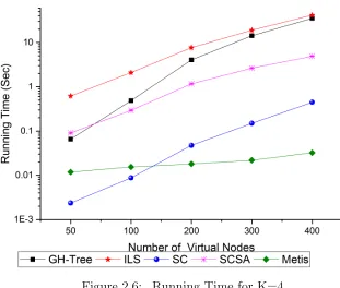
Figure 2.6 Running Time for K=4 . . . 30

Figure 2.8 Running Time for K=7. . . 31

Figure 2.9 Inter-cluster Traffic Ratio for Modular Pattern . . . 32

Figure 2.10 Running Time for Modular Pattern . . . 32

Figure 2.11 Inter-cluster Traffic Ratio for Waxman Model Pattern . . . 33

Figure 2.12 Running Time for Waxman Model Pattern . . . 33

Figure 2.13 Inter-cluster Traffic Ratio for BA-Model Pattern . . . 34

Figure 2.14 Running Time for BA-Model Pattern. . . 34

Figure 3.1 Reconfiguration of virtual network requests . . . 38

Figure 3.2 Augmented graph . . . 39

Figure 3.3 Maximum link utilization vs. number of reconfiguration events . . . . 58

Figure 3.4 Maximum node utilization vs. number of reconfiguration events . . . 58

Figure 3.5 InP revenue vs. number of reconfiguration events . . . 59

Figure 4.1 A service chain request (top) and corresponding walk on the topology graph (bottom) . . . 65

Figure 4.2 Walks under the two length functions for the example of Chapter 4.3.1. 67 Figure 4.3 Maximal congestion v.s. number of requests . . . 78

Figure 4.4 Maximal congestion v.s. number of requests . . . 78

(11)

Chapter 1 Introduction

1.1 Virtualization for the Networks

The Internet had achieved a great success in the past few decades. With billions of users and numerous services supported at the application layer, today’s Internet is truly reshaping and inter-connecting the world. Despite the fast growth both in size and the diversity of applications it supports, there has been significant slowing down when it comes to bringing in innovation to the Internet itself, as new architectures, protocols, and services are becoming increasingly difficult to integrate into today’s network. This is exemplified by the time and difficulties it takes to transit from IPv4 to IPv6, a process that started two decades ago, and remains far from completion [55].

The problem above is known as the Internet ossification problem, with multiple con-tributing factors. First, the dedicated and proprietary nature of networking devices re-quires non-trivial time and effort to make even small changes. Second, any changes to the existing network architecture would require consensus among all the Internet Service Providers (ISPs), making the implementation of a new architecture or protocol hard to realize. Moreover, the scale of today’s Internet adds more difficulties to it. As a result, nearly all the changes to the network has been achieved via the incremental deploy-ment [1].

(12)

services. Through the abstraction of the underlying infrastructure, it simplifies the effort to develop, deploy and maintain new services, thus lower the overall operational cost.

A number of networking architectures centering on virtualization have been proposed in this regards. Network Virtualization and Network Function Virtualization are two of them. In the subsequent paragraph, we shall briefly discuss the background on the two network paradigms, and the resource management problems in Network Virtualization and Network Function Virtualization environment.

1.1.1 Network Virtualization

Network Virtualization is seen as the enabler for the future generation of the networks. Through the virtualization techniques, it allows heterogeneous network to cohabit on the same infrastructure. Originally, network virtualization was proposed as a means to build a platform for the testing and evaluation of innovative network architectures or protocols on top of a legacy network environment, but now it is considered as one of the most promising paradigms for the next generation networks [1, 15, 16]. With network virtualization, the traditional role of ISPs is decoupled into two logical entities: Service Provider (SP) and Infrastructure Provider (InP) as shown in Figure 1.1.

In this context, InPs are responsible for the provisioning and management of the infrastructure, and offer their available resources as a service to SPs. By aggregating resources from multiple InPs, a SP can then create and deploy virtual networks on top of the leased infrastructure, and then deliver network services to the end users. The service provided to the users will be in the form of virtual networks (VNs).

Such a separation brings a number of benefits to network architectures, including but not limited to [6, 15, 16]:

• Heterogeneity: the same set of underlying physical infrastructure may support heterogeneous virtual networks, thus the services delivered to the users are no longer limited by the type of physical resources; in addition, the same VN may be mapped onto heterogeneous underlying physical infrastructures.

(13)

Figure 1.1: Virtual Network Environment [15]

as the virtualization provides an abstraction of the underlying physical resources, it simplifies the network management.

• Co-existence: with virtualization, multiple users can co-exist on the shared infras-tructure, and the service provider may decide how to pool the physical resources and how to aggregate requests so as to improve the overall utilization of the underlying infrastructure.

• Security and Isolation: the traffic of different users on a shared infrastructure can be isolated to the point where each user only has the view on its own slice of network. This ensures that traffic from one user will not interfere with that of another. Such an isolation will also help to enhance security of the system.

1.1.2 Network Function Virtualization

Network function virtualization (NFV) [34] is yet another networking paradigm that harnesses the power of virtualization. Through the virtualization of the conventional middleboxes (e.g., firewall, load balancer), NFV eases the difficulties in the developing, deploying and maintaining the networking services in today’s network.

(14)

hard to extend their functionalities. This makes it difficult for the service provisioning to accommodate a diverse and sometimes short-lived the network service requests. All those factors result in a long production cycle and a high operational expenditure which impedes the agility of deploying new services.

With the help of virtualization techniques, NFV relies on the commercial off-the-shelf hardware to replace the existing networking devices [29]. The most basic element in the NFV ecosystem is the Virtual Network Function (VNF), representing a single functional block. The network function can be implemented as the software and runs on the general purpose server. Based on demand, the service chain combines one or more network functions to accomplish the service objective. For a conventional way of service provisioning, packets need to go through the NFs in a given order, to deliver an end-to-end network service. Same will apply to the NFV environment, where packets are routed through VNFs sequentially. The VNFs will process those packets so as to deliver the network service.

Such a paradigm opens the door for network operators to implement both existing and future networking functions as software modules and consolidate them on the general-purpose commodity servers based on demand. This approach simplifies the deployment process and introduces flexibility in service provisioning.

1.2 Resource Management Challenges

Despite the promising outlook of the virtualization technology that can bring, one chal-lenge that both the network virtualization and network function virtualization face is the resource management problem, i.e., how to effectively allocate the available resource from the underlying infrastructure to the virtual requests. These problems are known as Virtual Network Embedding (VNE) and Network Function Virtualization Resource Allo-cation problems (NFV-RA) respectively. We shall discuss resource management problems in more details in the subsequent paragraphs.

1.2.1 Virtual Network Embedding Problem

(15)

underlying networks. Typically, the mapping of virtual network requests involves two sub-problems:

• Virtual Node Mapping, where a virtual node is instantiated on one physical node, and obtains the available resource from that substrate node accordingly • Virtual Link Mapping, where the traffic of one virtual link is routed along a

physical path, and the bandwidth is reserved accordingly. The endpoints of the physical path must be the substrate nodes where the virtual node is embedded upon.

Through the abstraction of the physical hardware, there are multiple ways to host one virtual network request. For example, for one virtual node, any substrate node with enough processing power can host that virtual node, while each virtual link may be along a path with enough bandwidth. This results in a large solution space for the potential mapping of the virtual network requests. However, it is to the interest of the network operator to obtain an efficient mapping of the virtual network requests.

Depend on the embedding objectives, an effective virtual network embedding strategy would help to deliver a better service to the end-users and to lower the operational cost. Those objectives under consideration may include enforcing QoS requirement [52], energy-efficiency [50] maintaining the survivability of the virtual network [49], load balancing [60] or maximizing revenue from existing infrastructure without service degradation [62].

The real challenge in solving virtual network embedding lies in the fact the VNE problem is NP-hard, i.e., it may not be possible to find an optimal solution within a reasonable amount of time. Even in the simplest case, where the network request remains static and is known in advance, this problem remains NP-hard [26]. How to design a resource allocation algorithm with a near-optimal performance becomes a critical issue.

(16)

1.2.2 Network Function Virtualization Resource Allocation

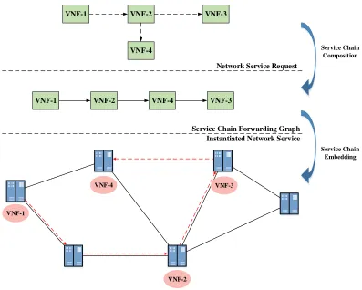
Unlike the service provisioning in a conventional network, where the network operator statically configures how the packets pass through the middle boxes, the service provision-ing under NFV environment can exploit the flexibility of the virtualization techniques to dynamically coordinate the virtual network functions and form the service chain. How-ever, how to allocate the resources from the underlying networks for Network Service (NS) requests also raise the issue of resource management.

The resource allocation problem can generally be depicted by two phases, the Service Chain Composition phase, and the Service Chain Embedding phase, as illustrated by the Fig. 1.2.

Within the NFV environment, some Network Services need to concatenate multiple VNFs to achieve the service goal. The NS request comes with the traffic demand and the specification on the necessary VNF types. Moreover, there may exist dependent relationships on the VNFs, meaning one type of the VNF needs to process a packet before the packet goes to another type of VNF. This procedure of dynamically concatenating multiple VNFs for the service deployment to meet the service goal is known as Service Chain Composition problems.

As the Service Chain Composition phase determines a service chain, taking it as an input, how to find an appropriate mapping of the service chain to the underlying infrastructure remains an issue. The process of finding an efficient mapping of a service chain to the underlying network is known as the Service Chain Embedding problems. Similar to the VNE problem, the Service Chain Embedding problem also involves the mapping of the virtual nodes and virtual links, and different embedding objectives and scenario would call for a different embedding scheme.

The two phases, Service Chain Composition and Service Chain Embedding, are both important to fulfill the goal of the service provisioning. The Service Chain Composition will strategically determine how the network service will be fulfilled and carried out, while Service Chain Embedding problem considers how to coordinate the physical resource to support the network service.

(17)

VNF-1 VNF-2 VNF-3

VNF-4

VNF-1 VNF-2 VNF-4 VNF-3

VNF-1

VNF-2

VNF-4 VNF-3

Network Service Request

Service Chain Forwarding Graph Instantiated Network Service

Service Chain Composition

Service Chain Embedding

Figure 1.2: NFA Resource Allocation

grammar, and greedily select the service chain that will minimize the traffic requirement. With a valid service chain in the form of the Service Chain Forwarding Graph, the Service Chain Embedding phase shall take the composed service chain as an input, and map it upon the physical network with a predefined service goal, such as end-to-end delay minimization [7] or provisioning cost minimization [41].

(18)

objec-tive to increase the request acceptance ratio. The service chain forwarding graph will be adjusted accordingly during the embedding process.

1.2.3 VNE and VNF-RA

From the discussions above, we can see that the VNE and the VNF-RA problem bear remarkable resemblance: both involve mapping the requests onto the substrate network with the finite capacity to meet the predefined objectives, which typically involves the mapping of virtual nodes and virtual links, while the process itself is NP-hard.

However, the difference exists both in terms of the request and the support from the underlying physical infrastructure.

When it comes to request, the virtual network request can be represented by a weighted graph, with the edge weights stand for the bandwidth requirement and node weight for the processing power demand. This is not the case for the VNF-RA problem, whose request consists of the source, destination, traffic demand, required types of the VNFs, and dependencies among the VNFs.

In the context of VNE, unless there is a policy constraint, such as geographical consid-eration, the virtual node can be mapped on to any substrate node. The network operator generally does not need to consider the interactions between two virtual network requests. This is not the case for the NFV-RA. For the VNFs required by an NS request, it can either reuse the existing VNFs or instantiate new VNFs. Thus, for the Service Chain Em-bedding, the network operator has to decide whether or not to instantiate new VNFs to accommodate new service request. And to embed the service chain, each virtual function node can only be placed onto the matching VNF instances.

In short, the NFV-RA is more complicated as it involves the composition of the service chain, decision on whether to instantiate new VNFs or to reuse the existing ones. However, in the embedding phase, the topology of the Service Chain Forwarding Graph is simpler, as it may either be a path or a tree, while the topology for the virtual network may be arbitrary weighted graph.

1.3 Contribution

(19)

First, we consider the problem of how to partition a virtual network request in a multi-domain environment so as to minimize the inter-multi-domain traffic. For the VNE problem, mapping virtual requests to multiple domains may be required for various reasons, includ-ing load balancinclud-ing [57], managinclud-ing the embeddinclud-ing cost [32], or policy requirements [19,46]. As inter-domain traffic is more expensive than intra-domain traffic, when we distribute a virtual network across two different domains, how to minimize the traffic across different domains becomes critical.

To this end, we consider the problem of virtual network request partitioning and present an algorithm inspired by spectral clustering to partition virtual network nodes under capacity constraints. Based on the Laplacian transformation of the matrix, the pair of virtual nodes with intensive traffic between them tend to stay close to each other on eigenspace. This allows us to partition the virtual network on the eigenspace. The clustering is done using the constraintk-means, which clusters the virtual network request on eigenspace with respect to the capacity of that cluster. As a further optimization, we use a simulated annealing-based algorithm to further refine the partitioning.

Next, we handle the problem of how to re-embed the virtual network so as to adapt to the dynamic changes in the network. Example to those changes include the dynamic arrival and departure of the request as well as the changes in the resource demands. If these dynamics are not taken into account and resource allocation is viewed as a purely static problem, the whole infrastructure may drift into an inefficient configuration that results in degraded performance for existing VNs and a higher rejection rate for subsequent VN requests [62].

Our approach is to design an algorithm to reconfigure the VN embedding on a pe-riodic basis. The mapping of virtual nodes and links to infrastructure resources will be updated in response to changes in VN requests. This is referred to as the virtual network reconfiguration (VNR) problem [21], and its objective is to improve resource utilization (for providers) and enhance performance (for users). Similar to the VNE problem, VNR is also concerned with the mapping of virtual nodes and links, but it also takes the existing configuration into account.

(20)

there is no bound on the number of virtual nodes to be migrated. Therefore, we decompose the problem into two phases, namely, virtual node selection and virtual node remapping. The first phase selects the virtual nodes to be migrated, while the second selects the new substrate nodes for the migrated virtual nodes. For the first phase, we solve the linear programming (LP) problem derived from the MIP. Specifically, we use a path-based formulation that achieves a near-optimal solution to the LP problem without intensive computation overhead. For the second phase, we use a Markov-chain based approach to select candid substrate nodes and solve a multi-commodity flow (MCF) problem for link reconfiguration.

Finally, we consider the problem of service chain routing problem, which is a sub-problem in the Service Chain Embedding phase for the NFV-RA sub-problem. The objective of the service chain routing problem is to route the user traffic along a path that starts at the source node, passes through the network locations where VNFs are implemented, and finally reaches the destination node. In an offline scenario, where all service requests are known in advance, service chain routing is NP-hard; this result follows from the fact that the unsplittable flow problem, which was proven to be NP-hard in [4], is a special case of the service chain routing problem. In practice, the service chain routing is an online problem: service requests may arrive at arbitrary times and they must be placed onto the network without prior knowledge of future requests. These conditions pose additional challenges in developing effective and efficient algorithms for the online problem.

In our work, we consider the service chain routing with the goal on minimizing the congestion in the network. Taking the online nature of the service request into account, we present a simple yet efficient online algorithm to minimize the maximum utilization. The algorithm we develop can achieve an O(logm) competitive ratio, in which m is the number of the edges in the substrate network. And we show that the competitive ratio is asymptotically optimal.

1.4 Structure of the Dissertation

The remainder of this dissertation is organized as follow:

(21)

Chapter 3 presents a virtual network reconfiguration strategy that aims to achieve load-balancing while minimizing the cost relocating virtual nodes.

Chapter 4 presents an online service chain routing algorithm for the network function virtualization with the objective to minimize the maximum system utilization.

(22)

Chapter 2 Virtual Network Request

Partitioning

As discussed in the previous chapter, the objective of virtual network request partitioning problem is to partition the virtual network requests into a set of clusters so as to minimize the inter-cluster traffic. The partitioning should be done in a way that the capacity constraint of each cluster would be satisfied. In this chapter, we develop a clustering algorithm based on spectral clustering to handle this problem. Previous work related to this topic is reviewed in Chapter 2.1. In Chapter 2.2, we formally define the virtual request partitioning problem, and then present an algorithm based on spectral clustering to solve this problem in Chapter 2.3. Finally, in Chapter 2.4, we present numerical result to demonstrate the effectiveness of this algorithm.

2.1 Related Work in Virtual Network Request

Par-titioning

(23)

graph of n nodes. By removing the k−1 least weight edges of this tree, a partition of the n nodes into k clusters is obtained that is close to optimal. One shortcoming of this method is that the resulting clusters may be highly imbalanced in terms of the number of nodes they contain.

The virtual network embedding problem across multiple domains has been considered in [40], where it was proposed to use iterative local search (ILS) to partition the virtual request. For this problem, ILS starts with a random clustering, following which a sequence of solutions is generated by randomly remapping some of the nodes to other clusters. Of these solutions, the one that improves upon the current solution the most is kept, and the algorithm iterates until a stopping criteria is met. Despite the simplicity of this method, it is hard to guarantee the quality of the solution within a limited time. In a related study, a general procedure for resource allocation in distributed clouds was presented in [19]. The objective was to select the data centers, the racks, and processors with the minimum delay and communication costs, and then to partition the virtual nodes by mapping them onto the selected data center and processors.

In [12], a series of spectral partitioning algorithms are reviewed and summarized. Most of those spectral partitioning techniques use the median of the Fiedler vector, the second smallest eigenvalue of the Laplacian matrix, to partition the graph into two parts. Then, by recursively applying this method, one can partition the graph into 2n, n≥1, parts. These algorithms have two limitations. First, the node weights related to load demands are not taken into consideration; consequently, the load may not be balanced well across the various clusters. Second, the number of clusters is limited to powers of two. In [30], a spectral partitioning based method that makes use of multiple eigenvectors of the Laplacian matrix is proposed. While this work considers the node weight balancing and makes use of multiple eigenvectors to produce a solution with a high-quality, it only partitions a graph into two, four or eight parts.

(24)

2.2 Problem Statement

We model the communication between virtual nodes as a traffic matrix T M = [tab]N×N,

where element tab represents the amount of traffic from virtual nodea tob. Each virtual

node is associated with a resource requirement Reqa, and each cluster k is associated

with a capacity threshold Capk.

With these definitions, partitioning the set of virtual nodes into K clusters so as to minimize the inter-cluster traffic can be formulated as the following Integer Linear Programming (ILP) problem:

minimize X

k

X

ab

tab(1−yabk ) (2.1)

subject to X

a

Reqaxak ≤Capk, ∀h (2.2)

xa_k+xb_k≤y_kab+ 1 ∀a, b, h (2.3)

y_kab ≤xa_k ∀i, j, h (2.4)

X

k

xa_k = 1, ∀a (2.5)

xa_k={0,1}, yab_k ={0,1} (2.6) The binary variable xa_k ∈ {0,1} here indicates if virtual node a is assigned to cluster k while binary variable y_kab ∈ {0,1} indicates if virtual nodes a and b are both mapped onto cluster k.

Constraint (2.2) ensures that the amount of resources assigned to each cluster will not exceed its capacity limit. Constraint (2.3) and constraint (2.4) guarantees consistency between decision variable x and y. Constraint (2.5) makes sure that virtual node a is assigned to exactly one cluster. This formulation is equivalent to the (k, v)-balanced partitioning problem, which is an NP-complete problem [2].

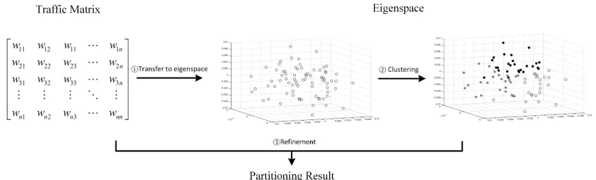
For the solving of the virtual request partitioning problem, we apply a spectral clus-tering based [53] approach. A high level idea of our approach is illustrated in the Figure 2. We aim to partition the virtual request that consists ofN nodes. Starting with aN-by-N traffic matrixT M, we compute the normalized Laplacian matrix Lsymof the given traffic

(25)

eigen-Algorithm 2.1 Spectral clustering based Virtual Request Partitioning Algorithm

Input:

T M: N ×N traffic matrix of virtual nodes K: number of clusters

Req: resource requirement vector of virtual nodes Cap: capacity vector of the clusters

Output:

The cluster to which each VNode belongs

1: Construct diagonal matrix D with daa =

PN

b=1tab

2: Compute unnormalized LaplacianLsym =D−1/2(D−T M)D−1/2

3: Obtain the eigenvector associated with the K smallest eigenvalues of matrixLsym

4: Let matrixU contain the above eigenvectors as columns

5: Letza be the vector associated withath row of U.

6: Cluster the points (za)|a=1...N under the capacity constraints Cap via Constrained

k-means

7: Refine the partitioning result by Greedy-Refinement based Simulated Annealing

vectors. Denote ath _{row of the matrix, a}_K _{dimensional vector, as} _z

a. The virtual node a

will be associated with za. We can think of the za as the coordinates for the virtual node

a on aK dimensional space, and the matrixZ as the collection of coordinates for theN data points. This K-dimensional space is referred as Eigenspace. With given property of the Laplacian matrix, the nodes that have higher traffic among them tend to stay closer on this Eigenspace. Thus, we can perform clustering for those data points (za)a=1,...,N.

(26)

2.3 Spectral Clustering Based Network Request

Par-titioning Algorithm

Spectral clustering [53] is used to find a set of clusters such that the edges between clusters have low weights (in this case, the weights would represent the pairwise traffic). An important feature of spectral clustering is that, unlike the conventional min-max flow approach, it can avoid the creation of imbalanced partitions whereby some clusters are assigned a much larger number of nodes than others.

2.3.1 EigenSpace

Given aN×N traffic matrixT M, the normalized Laplacian matrix is defined asLsym=

D−1/2_(D₋_T_)D−1/2_{, where}_D _{is a diagonal matrix with element} _d

aa =P_btab.

LetP1, . . . , PK be a partition of the set ofN virtual nodes into K sets (clusters), i.e.,

the sets Pk are pairwise disjoint and their union is {1, . . . , N}. Further, let ¯Pk be the

complement of setPk. We define the N Cut metric as:

N Cut(P1, P2, ..., PK) = K

X

k=1

cut(Pk,P¯k)

vol(Pk)

(2.7)

where the numerator represents inter-cluster traffic (i.e., between nodes in Pk and nodes

not in Pk) and the denominator denotes total traffic within cluster Pk.

Minimizing N Cut will result in a set of K clusters that have low inter-cluster traffic, while the presence of vol(Pk) in the denominator will prevent the creation of clusters

with few nodes, and hence, cluster sizes will not be highly imbalanced. The normalized Laplacian has the following property that allows us to find an approximate solution to the N Cut problem efficiently: for a given N-by-k matrix H, if we take hab as:

hab =

(

1/pvol(Pk) if vi ∈Pj

0 otherwise (2.8)

the following equation would hold [53]:T r(HT_LH_{) =} PN

i=1

cut(Pk,P¯k)

|vol(Pk)| =N Cut(P1, P2, ..., Pk).

(27)

mini-Figure 2.1: General Procedure for Virtual Request Partitioning

mizing N Cut as follows:

minimize T r(HTLH)

subject to HTDH =I (2.9)

hab ={1/

p

vol(Pk),0}

We can obtain an approximate solution to this problem in polynomial time by relaxing the last condition and taking Z =D−1/2H. The problem then becomes:

minimize T race(ZTLsymZ)

subject to ZTZ =I (2.10)

According to the Rayleigh-Ritz Theorem, the solution to problem 2.10 would be to take Z as the k smallest eigenvectors of Lsym, i.e. the eigenvectors corresponding to the k

smallest eigenvalues.

Let matrix Z be aN-by-k matrix that contains the above k eigenvectors as columns, and let zi be the vector associated with thea-th row of Z, and we take zi as coordinates

for the virtual nodes on the Eigenspace. The data points will stay close to each other in the Eigenspace if the traffic between them is high, and this will allow us to obtain the final solution using clustering algorithm. A formal proof of this property that established in the matrix perturbation theory is presented in [48].

To obtain the final solution, clustering will be performed to cluster the points (za)a=1,...,N

(28)

2.3.2 Constrained

K

-means

Conventional spectral clustering uses the k-means algorithm [44] to cluster the data points za. One drawback of the k-means algorithm is that it may converge to a solution

in which some clusters have very few data points while others are overloaded. Therefore, we use the constrained k-means algorithm proposed in [11]. Given a set of data points, the constrained k-means algorithm aims to find a set of cluster centers C1, C2, . . . , CK,

such that the sum of distances between each node and the center it is assigned to is minimal. Specifically, the problem solved in [11] is:

minimize N X a=1 K X k=1 xa_k·

1

2kza−Ckk 2 2 subject to N X k=1

xa_k = 1, ∀i; xa_k≥0, ∀i, ∀h. (2.11)

X

i

xa_k ≥τk, ∀k

In this formulation, xa_k is a selection variable denoting whether data point a belongs to cluster k. The last constraint is used to control the size of each cluster, i.e., to ensure that each cluster has size at least equal to τk.

In the virtual request partitioning problem, the resource requirement for each cluster should not exceed its capacity. To this end, we replace the constraint P

ix a

k ≥ τk with

P

iReqax a

k ≤Capk, and follow the iterative method proposed in [11].

Given N data points z1, z2, ..., zN, K cluster center points C1t, C2t, ..., CKt at iteration

t, and capacity limitCapk for cluster k, the cluster center for iterationt+ 1 is computed

(29)

Cluster Assignment. Given the fixed cluster center points Ck, find the selection

vari-ables so that the distance between the data points and the corresponding cluster center is minimized. minimize N X a=1 K X k=1 xa_k·

1

2kza−Ckk 2 2 subject to K X k=1

xa_k = 1, ∀a (2.12)

X

a

Reqaxak≤Capk, ∀k

xa_k ≥0, ∀a,∀k

Cluster Update. Compute the center point at iteration t+ 1 as:

C_kt+1 =







PN

i=1xak(t)za

PN

i=1xak(t)

ifPN

i=1x

a

k(t)>0

Ct

k otherwise

(2.13)

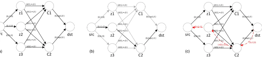
It was shown in [10] that cluster assignment is equivalent to the Minimal Cost Flow problem. We now show that this cluster assignment subproblem can be solved optimally within O(KN logN) time using a greedy approach.

We first reduce cluster assignment to the Min-Cost-Flow problem following the steps outlined in [10]. The supply from the source node (src) and the demand by sink node (dst) is equivalent to the total requirement PN

a=1Reqa. src is connected to all the data points (za)|a=1,...,N, and each data point is connected with all the cluster centers, while

cluster centers are connected todst. Each edge is associated with a weight tuple

(P rice, M aximumCapacity, F low). TheP ricefrom data points to cluster centers are set to the corresponding distance, while on other edges it is set to zero. TheM aximumCapacity from src to the data points is the resource requirement Reqa and from cluster center k

todstis Capk; on other edges, it is set to infinity. An example of the representation of a

(30)

Figure 2.2: Min-Cost-Flow view of clustering assignment subproblem

residual graph. An example can be found in Figure 2.2 (b) and (c).

A brief proof of optimality is as follows. Denote the iteration to augment flow on path i as ti. At ti, we augment flow on path i. For tj > ti, no negative cycle will form on

the residual graph involving the reversed path i, because the price of path j will be no less than of path i. Also, for path j with ti > tj, the price of path i is higher, hence a

negative cycle will be formed only when we take forward direction from on path j and backward oni, which is impossible. This is from the fact on pathj, the capacity onsrcto a data point or from cluster center otdstis depleted. In the former case, we cannot find a forward path fromsrcto the data point, so pathj is blocked, and no cycle will form. The same applies to the latter case when path i and j go through a different cluster center. If they pass through same cluster center, then, we cannot augment the flow on path i, because there is no available capacity from the cluster center todst, so no negative circle will form. In conclusion, no negative cycle can be found and the solution will be optimal.

At each step, denote the remaining capacity of cluster k asRmh

cap, and the remaining

resource requirement of each virtual node a as Rmi

res. Our constrained-k-means with

greedy cluster assignment algorithm is shown as Algorithm 2.2.

(31)

Algorithm 2.2 Constrained-K-Means

Input:

(za)a=1,...,N: data points formed by eigenvectors

K: number of clusters

R=r1, r2, ..., rN: resource requirement of VNodes

Cap=cap1, cap2, ..., capK: capacity of each cluster

Output: Selection indicator xa k

1: Iteration t←0, randomly initialize Ct k ∀k

2: Remaining resource requirement Rmreq←R

3: Remaining capacity Rmcap←Cap

4: while Ct+1 ₆₌_Ct _do

5: Clustering Assignment:

6: Compute pairwise distance between data points and cluster centers D =

{d11, d12, ..., dN K}

7: Ascending sort D to get Dasc ={d10, d02, ..., d0N∗K}

8: for j ←1to (N ∗K) do

9: Choose pointa and center point k associated with d0_j

10: if Rmi_req < Rmh_cap then

11: xa

k ←Rmireq/Reqa; Rmhcap ←Rmhcap−Rires; Rmires ←0

12: else

13: xa_k ←Rmh_cap/Reqa; Rmireq ←Rmireq−Rmhcap;Rmhcap ←0

14: end if

15: end for

16: Clustering Update:

17: update the center points according to (2.13)

18: t ←t+ 1

19: end while

(32)

Algorithm 2.3 Greedy Refinement Algorithm

Input:

K: Number of clusters

Initial assignment of VNodes to clusters Rmcap: Remaining capacity of each cluster

Cap: Maximum capacity for each cluster

Req: Resource requirement vector, remaining capacity

Output: Final assignment of VNodes to clusters

1: for a← selected virtual node do

2: assume node a∈ cluster k

3: ED[a]k|k=1,...,K ←0

4: for b←1 to N do

5: if nodeb ∈ clusterk0 then 6: ED[a]k0 =ED[a]_k0 +t_ab

7: end if

8: end for

9: k0 =argmax{ED[a]k s.t. capacity constraint}

10: move a from cluster k to k0

11: update Rmk_Cap0 12: end for

significantly greater than the number of clusters, we expect that this greedy rounding scheme will have only relatively small negative impact.

2.3.3 Partitioning Refinement

In order to improve upon the partition obtained by the Constrained-k-means algorithm, we employ a greedy refinement (GR) method that employs simulated annealing (SA). The GR algorithm is proposed in [37], which improves the Kernighan-Lin (KL) algorithm [38] to refine the bisection of a graph by iteratively swapping the pair of vertices that would most significantly reduce the edge cut until a local minimum is reached. The GR algo-rithm extends the KL algoalgo-rithm so as to handle vertex weights, refines the multi-way partitioning and improves the running time.

For completeness, we present the GR algorithm as Algorithm 2.3. Given an existing partition of the virtual nodes, the nodes are checked in a random order. Consider node a in cluster k. Denote ED[a]k as the total traffic between a and its neighbors that belong

(33)

Algorithm 2.4 New Point Generation

Input:

K: Number of clusters

nexc: Number of nodes to exchange

Initial assignment of VNodes to clusters Req: Resource requirement vector Cap: Maximum capacity vector

Output: P: Final assignment of VNodes to clusters

1: for a← random permutation from 1 to nexc do

2: node a∈ clusterk

3: if nodea has neighbor ∈cluster k0 and

4: Capk+Reqa < Cap0k then

5: move nodea from cluster k to k0.

6: end if

7: end for

8: for t ←1 to tref do

9: refine the partitioning via Greedy Refinement

10: end for

the highest value ED[a]k (or keeps it in the same cluster if it happens that h=l).

We now integrate this GR algorithm within a new point generation phase of SA: each time we randomly move a small number of nodes nexc from one cluster k to another k0,

such that (1) the node that is moved fromk tok0 should be on the “brink” (i.e., it should have at least one neighbor in the new clusterk0), and (2) this movement does not violate the capacity constraints of clusterk0. The exchange aims to introduce perturbation to the current solution so as to escape local minima. The procedure to generate new points is detailed in Algorithm 2.4. After the exchange is completed, we execute several iterations of the Greedy Refinement algorithm to refine the result.

The GR algorithm constructs a solution that represents a local optimum. The total outgoing weight of this solution is considered as the energy function for the SA algorithm. The SA algorithm will decide whether to accept this point or not. Since the solution passed to SA is already a local optimum point obtained by the GR algorithm, the SA moves around the local optimum points to find the final solution. This operation is more efficient than the naive implementation of randomly generating new points and letting the SA algorithm decide which solution to take.

(34)

computing the eigenvectors of the graph Laplacian, constrained k-means, and graph re-finement. The computation of the eigenvectors can be completed inO(N3_{) time. For the} constrainedk-means, the clustering assignment subproblem can be solved inO(KNlogN) time, where K is the number of clusters, and the cluster update problem can be solved in O(kn) time. Let tc be the number of iterations for constrained k-means to converge;

then, the total running time for the constrained k-means is O(KtcN lgN). Using an

ad-jacency table, each iteration of the refinement phase can be completed in time O(E). If tr iterations are needed, the refinement phase takes timeO(trE). Overall, this algorithm

runs in O(N3+KtcNlogN +trE) time.

2.4 Experiments and Evaluation

We now present the results of experiments we have conducted to evaluate the perfor-mance of spectral clustering (SC)-based algorithms. We use two methods to refine the partitioning: solely based on the GR algorithm (referred to as SC) as well as the SA-based refinement approach (SC-SA) we described previously in this chapter. We compare the results to those obtained using a Gomory-Hu tree [46], the Metis [36], and the ILS method [40].

To evaluate the performance of our approach, we generate topology as follow: the vir-tual node is pairwise connected, and each node and link is assigned a weight to represent the resource and traffic requirements, respectively, and we also specify the maximum available capacity for each cluster. For each randomly generated topology, the vertex weight is uniformly distributed in (1,2), the edge weight is uniformly distributed in (5,20). Our goal is to partition the network into K = 3,4,7 clusters. For each cluster, we set the maximal capacity to 105% of the average weight of each cluster, i.e. the weight we place onto each cluster if we can have a perfect load balancing of the nodes. For the ILS algorithm, we set the number of iterations to be 5×104 and for each iteration, exchange 40% of nodes in each cluster. We also set nexc = 15 for new point generation phase in

(35)

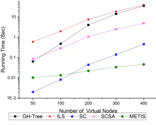
Figures 2.3 and 2.4 plot the ITR and running time, respectively, against the number of virtual nodes and forK = 3 clusters. For the SA algorithm, we set the initial temperature toT emp= 104 _{and the maximum number of iterations to 600. We observe that spectral} clustering with SC-SA method is strictly better than the other algorithms in terms of inter-cluster traffic minimization. Compared with Metis, it reduces the inter-cluster traffic by 6-9% percent, with an average improvement of 8.3%. Compared with Gomory-Hu tree (respectively, ILS), inter-cluster traffic is reduced by as much as 11% (respectively, 9.7%), with an average improvement of 10% (respectively, 8.2%). Also, compared with the SC only, SC-SA based refinement produces an improvement of 1.6% on average. In terms of running time, with a small number of virtual machines, the SC algorithm has the similar performance with Metis while the running time for SC-SA stays close to the Gomory-Hu tree method, about one magnitude larger than the two above, while ILS takes still one magnitude longer. When there are more virtual nodes, we see that the GH-Tree have a similar performance with the ILS, about an order of magnitude larger than the SC-SA, while SC takes less running time by an order of magnitude than SC-SA, and Metis takes yet another order of magnitude less than SC.

The second set of simulation experiments is to partition the virtual request into K = 4 clusters, and the results are shown in Figures 2.5 and 2.6. We kept the initial temperature for SA to T emp = 104 and the maximum number of iterations as 600. The SC algorithm produces clustering solutions that, in terms of inter-cluster traffic, outperform those produced by the Metis, Gomory-Hu tree, and ILS schemes by 4.5%, 6.5%, and 4.7%, respectively, on average. The SC-SA algorithm further reduces inter-cluster traffic by 1.1% on average, compared to SC. The running time results are similar to the experiments with K = 3 above.

Finally, Figures 2.7 and 2.8 plot the results of the third set of simulation experiments where we set K = 7. The initial temperature for SA was set to T emp = 105 and the maximum number of iterations to 600. The results are similar to those of the first two experiments, in that, on average, the SC algorithm performs 4.5% better than Metis, 6.1% better than Gomory-Hu tree, and 4.8% better than ILS. Also, compared with SC, the SC-SA algorithm reduces inter-cluster traffic by a further 0.7% on average. In terms of running time, the relative behavior of the five algorithms is also similar to the last two experiments.

(36)

SA refinement produces the best solutions in terms of minimizing the inter-cluster traffic. It also compares favorably to existing clustering approaches based on ILS and Gomory-Hu tree, in terms of running time. When we compare with METIS, we found out its performance is at trade-off with Metis: the spectral clustering based algorithm achieve a better performance in minimizing the inter-cluster traffic, while Metis achieves a lower execution time.

To further evaluate the performance of our proposed algorithm, we compare the per-formance of our algorithm with METIS on three different kind of topologies with different partitioning settings. Among entire set of simulation, we selectively present three groups of evaluation results that would illustrate the performance.

First, we evaluate the result on random modular graph [33]. This intends to capture the pattern that the communication took place within one groups is more intensive than that of others. We assume the topology contains 20 clusters with equal size, and the probability of connecting one pair of node within the same cluster is 80%, while connecting one pair node from two different cluster is 20%. We generate the topology using this model, and the traffic on each link follows a Gaussian distribution, with a mean of 100 and variance of 25. We partition the generated graph into 3 clusters, and capacity constraint is set to 120% of the average. This setting for the capacity constraint tries to capture the condition that abundant computing resources in the underlying network is provided for each cluster such that a more flexible partitioning of the virtual request is allowed. The result is presented in the Figure 2.9.

In this set of simulation, we can see that inter-cluster traffic is minimized by SCSA with an additional 2.7% on average when compares with METIS. However, when we compare the result between METIS and SC, we can see that METIS achieves a better result on smaller request by as much as 9%, while the SC achieves a better result on a larger request by around 3%. On average, METIS can bring about 3% of improvement than SC for traffic minimization.

(37)

β are two parameters that will define the connectivity pattern. More specifically, α will define the overall connectivity probability, a higherα will result in a denser connectivity, while β restricts the probability of connection based on the distance, i.e. with a larger β tends to increase the chance of connection for a pair of nodes that are far from each other, while a lower β tends to prevent such connection. In this experiment, we use L = 100, α= 0.05, andβ = 0.3 to define the connectivity of the virtual request. For the partition-ing settpartition-ing, we divide the virtual request into 4 clusters with different capacities, each cluster with 20%, 20%, 30%, 30% of the total weight of the request. Maximum violation for the capacity is defined to be 5%. This setting may comply with the situation where the distribution of the computational resource is imbalanced, such as heterogeneous re-sources, or imbalanced workload on different domains. The simulation setting is shown in Figure 2.11.

As we can see from the simulation results, the SCSA achieves an improvement of 5% compared with METIS for ITR minimization, while SC delivers a 2.5% improvement compared with METIS.

Finally, we evaluate this algorithm on the virtual request whose degree distribution exhibits power law, which characterizes the degree distribution of router-level and AS-level Internet graphs [22]. We use Barab´asi-Albert (BA) model [5] to obtain a topology that follows the power-law. It starts with a small connected component, and then prob-abilistically attach new vertex to the existing vertex following preferential attachment, i.e. the likelihood of connection depends on the degree of the existing vertex. We start with 5 connected vertex and ended up with a topology consisting of 50 to 400 vertices. We partition the graph into four clusters with equal capacity, while allows a cluster to exceed its capacity limit by 5%, the simulation result is shown in Fig.2.13.

Compared with METIS, the simulation result suggests an average improvement of 34% in term of ITR minimization for SCSA, with a maximum improvement of 43%, while SC brings forth an improvement of 14% compared with METIS on average.

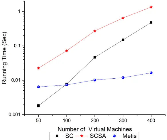
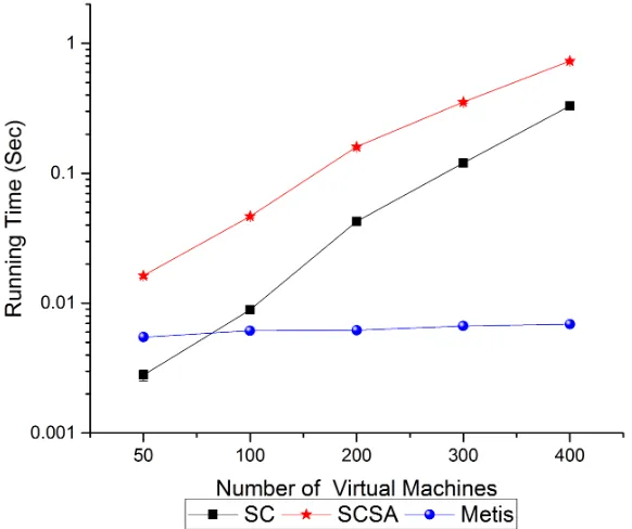
The running time on three different type of topology is similar to the previous set of simulation. As it is shown in Fig. 2.10, Fig. 2.12 and Fig. 2.14. METIS requires less execution time compared with SCSA, by two orders in general. Compared with SC, we see that their performance is similar on a request with small scale, while on a larger request, METIS will still work better.

(38)

(39)

Figure 2.3: Inter-cluster Traffic Ratio for K=3

(40)

(41)

(42)

Figure 2.9: Inter-cluster Traffic Ratio for Modular Pattern

(43)

Figure 2.11: Inter-cluster Traffic Ratio for Waxman Model Pattern

(44)

Figure 2.13: Inter-cluster Traffic Ratio for BA-Model Pattern

(45)

Chapter 3 Virtual Network Reconfiguration

with Migration Cost Consideration

In this chapter, we present the design of an algorithm that will handle the online nature of the virtual network requests by reconfiguring the virtual network requests. Such a re-configuration may help to improve network performance by remapping a subset of virtual nodes or links to better align the allocation of resources to current network conditions. In Chapter 3.2, we formally define the Virtual Network Reconfiguration (VNR) problem and introduce the augmented graph model we use in developing the formulation. We present the algorithm we have developed for the VNR problem in Chapter 3.3, and we evaluate its performance in Chapter 3.4.

3.1 Related Work in Virtual Network

Reconfigura-tion Problem

(46)

A proactive reconfiguration algorithm, referred to as global marking algorithm, was proposed in [62]. In the reconfiguration phase, the workload of the substrate nodes and links is examined. If a given substrate node or link is overloaded, then all virtual nodes and virtual links mapped on top of that particular substrate node or link, respectively, are marked for remapping. During the remapping phase, marked virtual nodes and links are re-assigned to the SN. This approach may incur unnecessary reconfigurations: often, only a fraction of the virtual nodes on a stressed substrate node need to be migrated, whereas this method tends to reconfigure all of them. Also, for congested substrate links, solely reconfiguring the mapping of the virtual links without migrating the virtual nodes causing the overload may not fully alleviate the congestion.

Another reconfiguration scheme to maximize InP revenue was proposed in [51]. This approach takes into account the migration overhead so as to limit the service disruption caused by reconfiguring the virtual nodes. Reconfiguration is triggered whenever a VN request is blocked, and follows the solution of a MIP problem. Since this method relies on solving the MIP problem, it may not scale to large problem sizes or may not be appropriate whenever a low reconfiguration delay is required.

Based on the observation in [21] that VN request rejection is mainly caused by band-width shortage, a reactive VN reconfiguration algorithm was presented in [18]. The al-gorithm aims at improving the VN request acceptance rate while limiting the number of virtual nodes to be migrated, so as to minimize the overall reconfiguration cost. Virtual nodes are selected for migration based on the number of congested links along which they route their traffic. Selected virtual nodes are iteratively reconfigured until either the incoming VN request is successfully embedded or the number of virtual nodes re-configured exceeds the given threshold. This work solely considers congested links and does not account for overloaded substrate nodes. Also, it does not take into consideration the magnitude of traffic demands originating/terminating at the virtual nodes. This may result in a situation whereby virtual nodes with little traffic (and hence, small impact on the SN) are selected for migration just because they happen to use congested paths. As an extension to the work in [21], a VN reconfiguration strategy was developed in [18] to handle the scale-up/down of VN requirements requested by users. This study used a genetic algorithm to minimize the combined cost of embedding and reconfiguration.

(47)

SN, i.e., whenever substrate nodes and/or links are added or removed. The objective is to reconfigure the VN such that delay constraints are preserved while migration overhead is minimized. To this end, a heuristic algorithm was proposed to relocate virtual nodes that are affected by the changes or violate the delay constraints.

3.2 Problem Definition

We model the SN as a weighted, undirected graph Gs = (Vs, Es). The vertices of Gs stand for the substrate nodes, while the edges of Gs represent the substrate links. Each node A and edge (A,B) on Gs _{are weighted, and we let} _Cap

A denote the resource (e.g.,

CPU) capacity of the substrate node A, and CapAB denote the bandwidth capacity of

substrate link (A,B).

Likewise, we model a VN as a weighted, undirected graph Gv _{= (V}v_{, E}v_{), whose}

vertices and edges represent virtual nodes and links, respectively. The weight Reqa of

vertex a reflects the resource (e.g., CPU) requirement of the virtual node, while the weight tab denotes the traffic demand of the virtual link (a, b)

In addition, each virtual node may specify additional constraints, including the type of the substrate nodes they may be mapped onto, geographical constraints, etc., such that a virtual node may be placed only on a specific group of substrate nodes. We denote the set of substrate nodes that may support a virtual nodea as Θ(a)⊆Vs_.

We assume that there exists a mapping of virtual nodes and links to the substrate network, F : Gv _→ _Gs_{. We also assume that the resource requirements} _Req

a and

traf-fic demands tab of the VNs evolve over time such that the current mapping F is not

representative of the current state of the network. Although our work is agnostic with respect to how reconfiguration is triggered (e.g., whether it is performed periodically or is initiated as soon as a performance measure crosses a predefined threshold), our focus is on updating the mapping F to align it with current network conditions.

3.2.1 Reconfiguration Objectives

(48)

Figure 3.1: Reconfiguration of virtual network requests

low and minimize service disruption. A reconfiguration example is shown in Figure 3.1. The top part of the figure shows the two VN requests and the original embedding of the requests onto the substrate network, whereas the bottom part of the figure shows the new embedding of the two requests after reconfiguration has taken place.

We view this VNR problem as a multi-objective optimization problem, with three metrics to be minimized: substrate link utilization, substrate node workload, and the number of virtual nodes to be migrated. Specifically, we take link utilization as the primary objective and bound the other two, such that we formulate the goal in this form:

Minimize the maximum link utilization λ, under two constraints: resource utilization of each substrate node does not exceed ρλ, and the total number of virtual nodes being migrated does not exceed a threshold M.

(49)

Figure 3.2: Augmented graph

3.2.2 Augmented Graph

Our problem formulation makes use of the augmented graph presented in [17]. We start with the graph Gs _{that represents the substrate network and follow these steps to}

con-struct the augmented graph Gaug _{(refer also to Figure 3.2). For each substrate node} _A,

we create a mirror node A0, as well as an edge (A, A0) with weight equal to the capacity of node A, CapA. For each virtual node a, we also create a corresponding node in the

augmented graph. Recall that Θ(a) is the subset of substrate nodes to which virtual node a may be mapped. Therefore, for each substrateA∈Θ(a), we create an edge (a, A0) be-tween the virtual nodeaand the mirror node of A. For instance, in Figure 3.2 we assume that Θ(a) = {A, D}, hence the augmented graph contains the edges (a, A0) and (a, D0). The capacity of these edges is set to infinity.

In addition to the weight (capacity), we associate a cost with each edge in the aug-mented graph, as follows: the cost on all edges except the ones between virtual nodes and mirror substrate nodes is zero. If, in the current configuration, a virtual node a is mapped on, say, substrate node A, then the cost of edge (a, A0) is also zero. Otherwise, the cost of the edge (a, D0), A6=D∈Θ(a), is the reciprocal of the total traffic of virtual nodea, i.e., 1/P

(50)

3.2.3 MIP Formulation

Using the augmented graph defined above, we formulate the VNR problem as the follow-ing mixed-integer programmfollow-ing (MIP) problem.

Decision Variables:

xa_A: binary variable, indicating whether virtual nodea is mapped onto substrate nodeA. f_ABab : flow variable, indicating the fraction of traffic between virtual nodes a and b that is mapped onto substrate link (A, B).

MIP Formulation:

min λ (3.1)

s.t.

X

A∈Θ(a)

f_aAab0 −

X

A∈Θ(a)

f_Aab0_a = 1,

∀a, b∈Vv,(a, b)∈Ev (3.2)

X

B∈Θ(b) f_bBab0−

X

B∈Θ(b)

f_Bab0_b =−1,

∀a, b∈Vv,(a, b)∈Ev (3.3)

X

A∈VS

f_ABab − X

A∈VS

f_BAab = 0,

∀a, b∈Vv,(a, b)∈Ev, A, B ∈Vs (3.4)

X

(a,b)∈Ev

tabfABab ≤λCapAB, ∀A, B ∈Vs (3.5)

X

a∈Vv

ReqaxaA ≤ρλCapA, ∀A∈Vs (3.6)

X

b∈Vv

f_aAab0 =

X

b∈Vv

xa_A, ∀a, b∈Vv, ∀A∈Vs (3.7)

X

a∈Vv

(1−xa_A)≤M, ∀a∈Vv, A=Ext(a) (3.8)

X

A∈Θ(a)

xa_A= 1, ∀a∈Vv (3.9)

0≤f_ABab ≤1 (3.10)

(51)

Remarks:

The objective of the MIP is to minimize the maximum utilization of any link in the SN.

Constraints (3.2)-(3.4) are the flow related constraints. Assume there exists a virtual link (a, b) between virtual nodes a and b, i.e., that the traffic between them tab > 0.

Constraint (2.2) specifies that all traffic between a and b must pass pass through the mirror nodes that are connected to virtual node a in the augmenting graph. Similarly, constraint (2.3) ensures that all traffic will be routed to virtual node b via mirror nodes connected to that node in the augmented graph. Constraint (2.4) is the flow conservation constraint, and ensures that the net traffic in and out of a substrate node is zero.

Constraints (3.5) and (3.6) are the substrate link and node capacity constraints, respectively. Constraint (3.5) states that the total amount of traffic on a substrate link may not exceed λ times its capacity, while constraint (3.6) asserts that the resource requirement on a substrate node may not exceed ρλ times its capacity.

Constraint (3.7) maintains consistency between decision variablesxandf, as it guar-antees that, if virtual nodeais mapped onto substrate nodeA, then all traffic associated with a will go through the augmented link between node a and the mirror node A0.

Constraint (3.8) ensures that the number of virtual nodes to be migrated does not exceed the threshold M. Here, Ext(a) stands for the substrate node upon which virtual nodeais mapped prior to reconfiguration. If, after reconfiguration, virtual node ais still placed upon substrate node A = Ext(a), then the term (1−xa

A) will be 0. Thus, the

sum on the left hand side of the constraint equals the number of virtual nodes that are remapped due to reconfiguration.

Constraint (3.9) ensures that each virtual node is mapped to exactly one substrate node, while the last two constraints define the range of the decision variables.

3.3 Reconfiguration Algorithm

Since VNR is an NP-hard problem, to tackle it efficiently we decompose it into two subproblems, namely, virtual node selection and virtual node remapping, described below.

Virtual Node Selection. Inspired by the work of [17], we use an LP relaxation based ap-proach to select the virtual node to be migrated. First, we relax the integral constraints on variablesxa

(52)

Hence, virtual node selection is carried out by jointly considering the load on substrate links and nodes. Although LP problems are solvable in polynomial time, the computation time may be prohibitive for large-scale networks. To overcome this difficulty, we propose an approximation algorithm to obtain a near-optimal solution with small computation overhead. As a result, the delay to reach a reconfiguration decision may be kept low.

Once the LP problem is solved (optimally or using the approximation algorithm), we ascending sort variables xa_A, where A = Ext(a). Note that we can think of xa_A as the likelihood that virtual node a is to remain in the same substrate node A. Consequently, we mark theM virtual nodes with the smallest value of xa_A as the nodes to be migrated.

Virtual Node Remapping: We have developed an algorithm based on a random walk on a Markov chain to filter substrate nodes for the virtual nodes selected in the solution to the previous subproblem, and use a MIP to map them back to the substrate network. This remapping phase takes into account load balancing across the substrate nodes and links.

3.3.1 Virtual Node Selection

As we mentioned above, solving a large-scale LP problem is computationally expensive, and may result in long reconfiguration delays that are not acceptable in an online scenario such as the one we are considering. Furthermore, we note that solving the LP problem exactly isnot necessary: our focus is not on the exact values of variablesxa

Abut rather on

their relative values, since the goal is to rank virtual nodes based on their likelihood to be migrated. With this in mind, we build upon the work of [35] to design an approximation algorithm to obtain a near-optimal solution to the relaxed LP.

Path-based Formulation

In order to develop the approximation algorithm, we first present a path-based formula-tion that is equivalent to the link-arc MIP formulaformula-tion (3.1)-(3.11), and relax the integral constraints. The path-based formulation is based on the observation that, by construc-tion, the augmented graph imposes a connection between the mapping of a virtual node and routing. Specifically, if there is traffic flow between a virtual node a and a mirror nodeA0, this implies a mapping ofa onto substrate node A.

(53)

capacity of the corresponding substrate node). Similarly, we denote edges representing substrate links ase, and their capacity asc(e). LetPab be the set of paths between virtual

nodesaandb, andTadenote the traffic originating at virtual nodea, i.e.,Ta =P_b∈Vvtab.

We define the decision variables x(p) as the amount of flow routed along path p. We also define ra

p as a normalization factor which builds an association between the routing of

the flow and the mapping of virtual nodes to substrate nodes: if routing flow along path p indicates that virtual node a is mapped onto substrate node A, then ra_p = Reqa/Ta.

Note also that, since the flow on a path p indicates the substrate node to which the virtual nodes generating that flow are mapped, it also indicates whether or not these virtual nodes are to be migrated. Therefore, we introduce binary parameter ηa_p defined as follows: if path x(p) indicates that virtual node a is to be migrated, then ηa

p = 1,

otherwise ηa p = 0.

Based on these observations, we have the following path-based LP formulation of the relaxed version of the above MIP problem.

LP Formulation:

min λ (3.12)

s.t.

X

p:e∈p

x(p)≤λc(e), ∀e ∈Es (3.13)

X

p:eA_∈_p

r_pax(p)≤ρλc(eA),∀A∈Vs (3.14)

X

p∈Pab

x(p)≥tab, ∀a, b∈Vv (3.15)

X

p,a

η_pa Ta

x(p)≤M (3.16)

x(p)≥0, ∀p. (3.17)

Resource Allocation in Virtual Network Environments.

ABSTRACT

DEDICATION

BIOGRAPHY

ACKNOWLEDGEMENTS

TABLE OF CONTENTS

LIST OF FIGURES

Chapter 1

Introduction

1.1

Virtualization for the Networks

1.1.1

Network Virtualization

1.1.2

Network Function Virtualization

1.2

Resource Management Challenges

1.2.1

Virtual Network Embedding Problem

1.2.2

Network Function Virtualization Resource Allocation

1.2.3

VNE and VNF-RA

1.3

Contribution

1.4

Structure of the Dissertation

Chapter 2

Virtual Network Request

Partitioning

2.1

Related Work in Virtual Network Request

Par-titioning

2.2

Problem Statement

2.3

Spectral Clustering Based Network Request

Par-titioning Algorithm

2.3.1

EigenSpace

2.3.2

Constrained

K

-means

2.3.3

Partitioning Refinement

2.4

Experiments and Evaluation

Chapter 3

Virtual Network Reconfiguration

with Migration Cost Consideration

3.1

Related Work in Virtual Network

Reconfigura-tion Problem

3.2

Problem Definition

3.2.1

Reconfiguration Objectives

3.2.2

Augmented Graph

3.2.3

MIP Formulation

3.3

Reconfiguration Algorithm

3.3.1

Virtual Node Selection