Ant Lion Optimization Algorithm for Solving Non-convex Economic Load Dispatch

Ant Lion Optimization Algorithm for Solving

Non-convex Economic Load Dispatch

Neilcy Tjahja Mooniarsih1, Sutrisno2, Dwi Handoko3, Muhammad Saleh4, Hardiansyah5

Department of Electrical Engineering, University of Tanjungpura, Indonesia1, 4, 5

Department of Mechanical Engineering, State Polytechnic of Pontianak, Indonesia2, 3

ABSTRACT:This paper presents a new technique to solve non-convex economic load dispatch problem using ant lion

optimization (ALO) algorithm. ALO is a newly depeloved population-based search algorithm inspired hunting mechanism of ant lions. The performance of ALO algorithm is tested for economic load dispatch problem of 6-unit and 40-unit test systems with incremental fuel cost functions taking into account the valve-point effects. Simulation results shows that the proposed method has good convergence property and better in quality of solution than other algorithms reported in recent literature.

KEYWORDS: Ant lion optimization algorithm, economic load dispatch, valve-point effects.

I. INTRODUCTION

The economic load dispatch (ELD) problem is one of the fundamental issues in power system operation and control, where the total required load is distributed among the generation units in operation. The objective of ELD problem is to minimizing total generation cost while satisfying load and operational constraints [1]. Various methods and investigations are being carried out until date in order to produce a significant saving in the operational cost. Generally, fuel cost function of a generator is represented by single quadratic function, but a quadratic function is not able to show the practical behavior of generator. The ELD problem is a non-convex and nonlinear optimization problem. Due to ELD complex and nonlinear characteristics, it is hard to solve the problem using classical optimization methods such as gradient method, lambda iteration method, Newton’s method, linear programming, Interior point method and dynamic programming [2].

In the past years many optimization algorithms are being developed to solve ELD problems such as genetic algorithm (GA) [3, 4], tabu search (TS) [5], simulated annealing (SA) [6], neural network (NN) [7, 8], evolutionary programming (EP) [9]-[11], biogeography-based optimization (BBO) [12], artificial bee colony (ABC) [13], and particle swarm optimization (PSO) [14]-[18].

Recently, a new meta-heuristic search algorithm, called ant lion optimization (ALO), has been developed by Mirjalili in 2015 [19]. In this paper, ALO algorithm has been used to solve ELD problem considering valve-point effect and transmission loss. The feasibility of the proposed method has been demonstrated on 6-unit and 40-unit test systems. The results obtained with the proposed algorithms were compared with other optimization results reported in literature.

II. PROBLEM FORMULATION

The main purpose of the ELD problem is to determine the optimal combination of power plants that minimize the total cost of generation while meeting the equality and inequality constraints

.

The fuel cost curve for each unit is assumed to be approximated by segments of quadratic functions of the active power output of the generator. For a given power system network, the problem may be explained as optimization (minimization) of total fuel cost as defined by (1) under a set of operating constraints.

_

_





 

  



n

i

i i i i i n

i i i

T F P aP bP c

F

1 2

1 )

where FT is total fuel cost of generation in power system ($/hr), ai, bi, and ci are the cost coefficient of the i-th generator, Pi is the power generated by the i-th unit and n indicates the number of generators.

2.1. Active Power Balance Equation

For the balance of power, an equality constraint should be satisfied. The total generated power should be the same as total load demand plus the total transmission loss.

Loss n

i i

D P P

P 

_



1

(2)

where PD is the total load demand and PLoss is total transmission loss. The transmission losses PLosscan be calculated by using B matrix technique and is defined by (3) as,

00 1

0 1 1

B P B P B P

P _i

n

i i j

ij n

i n

j i

Loss 

 







  

(3)

where Bij is coefficient of transmission losses and the B0iand B00 is matrix for loss in transmission which are constant under certain assumed conditions.

2.2. Minimum and Maximum Power Limits

The output power of each generator should lie between minimum and maximum limits, so that P_imin _P_{i }P_imax for i_1,2,_,n

(4)

whereP_iminandP_imaxare the minimum and maximum outputs of the i-th generator, respectively. 2.3. Valve-Point Effects

The fuel cost function with the valve-point effects of the thermal generating unit are taken into consideration in the ELD problem by superimposing the basic quadratic fuel-cost characteristics with the rectified sinusoidal component as follows [15]:

_

_













 

      



n

i

i i i i i i i i i n

i i

T F P aP bP c e f P P

F

1

min 2

1

sin )

( (5)

where FT is the fuel cost function of generating unit in ($/hr), ei, fi are fuel cost coefficients of the i-th generating unit reflecting valve-point effects.

III. ANT LION OPTIMIZATION (ALO)

Ant Lion Optimizer (ALO) is a novel nature-inspired algorithm proposed by Sayedali Mirjalili in 2015 [19]. The ALO algorithm emulates the hunting mechanism of antlions in nature. There are five main steps of the algorithm such that random walk of ants, building traps, entrapment of ants in traps, catching preys, and re-building traps. Antlions belong to the Myrmeleontidae family and Neuroptera order (net-winged insect). The lifecycle of antlions include two main phases: larvae and adult. They mostly hunt in larvae and undergo reproduction during adult. An antlion larvae digs a cone-shaped pit in sand by moving along a circular path and throwing out sands by using massive jaws. After digging the trap, the larvae hides underneath the bottom of the cone and waits for insect to be trapped in the pit. When a prey in caught, it will be pulled and consumed. After that, the antlions throw the leftovers outsode the pit and improve the pit for the next hunt.

3.1. Random Walk of Ants

The ALO algorithm imitates the interaction between ant lions and ants in the trap. For such interaction models, ants are required to move over the search space and antlions are allowed to hunt them and become fitter using traps. Since ants move stochastically in nature when searching for food, a random walk is chosen for the modeling ants’ movement as follows:

] 1 ) ( 2 ( , , 1 ) ( 2 ( , 1 ) ( 2 ( , 0 [ )

(t  cums rt1  cums r t2  cums rtn 

X  (6)

            5 . 0 , 0 5 . 0 , 1 ) ( rand if rand if t

r (7)

The position of ants are stored and used during optimization process in the following matrix:

               d n n n d d ant ant ant ant ant ant ant ant ant ant M , 2 , 1 , , 2 2 , 2 1 , 2 , 1 2 , 1 1 , 1       (8)

where, Mant is matrix to save the position of each ant, antij is value of j-th variable (dimension) of i-th ant, n is number of ants, and d is number of variables.

During optimization process, matrix Mantwill save the position of all ants (variables of all solutions). Random walk of ants are being normalized to keep them moving within the search space using the following equation:

i i t i t i i i t i t i c a d c d a X X       ) ( ) ( )

( ₍₉₎

wherea_iindicates the minimum of random walk of i-th variable, d_iis the maximum of random walk in i-th variable, t

i

c is the minimum of i-th variable at t-th iteration, and t i

d indicates the maximum i-th variable at t-th iteration.

3.2. Trapping in Ant Lion’s Pits

The following equations are used to represent mathematically model of antlions pits. t

t j t

i Antlion c

c   (10)

t t j t

i Antlion d

d   (11)

where t

c is the minimum of all variables at t-th iteration, t

d indicates the vector including the maximum of all variables at t-th iteration, t

i

c is the minimum of all variables for i-th ant, t i

d is the maximum of all variables for i-th ant, and t

j

Antlion shows the position of the selected j-th antlion at t-th iteration.

3.3. Building Trap

Ant lion’s hunting ability is modeled by roulette wheel operator for selecting ant lions based on their fitness during optimization. This mechanism gives great probabilities to the fitter ant lions for catching preys.

3.4. Sliding Ants towards Ant Lion

Ant lions are capable to build traps proportional to their fitness and ants are necessary to move randomly. Once the ant is in the trap, ant lions will shoot sands outwards the center of the pit. This behavior slides down the trapped ant in the trap. The radius of ants’s random walks are represented as (12) and (13),

I c c

t t

 (12)

I d d t t  (13)

where I is a ratio, t

c is the minimum of all variables at t-th iteration, t

d indicates the vector including the maximum of all variables at t-th iteration.

3.5. Catching Prey and Re-Building the Pit

Last phase of hunt is when ant reaches the bottom of the pit and being trapped in the ant lion’s jaw. The ant lion attracts the ant inside the sand and consumes its body. It is assumed that catching prey occur when ants become fitter (goes inside sand) than its corresponding ant lion. Ant lion is required to modernize its location to the latest position of the hunted ant to improve its chance of catching new prey.

It is represented by the following equation:

) (

) (

, t

j t

i t

i t

j Ant if f Ant f Antlion

Antlion   (14)

where t is the current iteration, t j

Antlion shows the position of selected j-th antlion at t-th iteration, and t i

Ant indicates the position of i-th ant at t-th iteration.

3.6. Elitism

The best ant lion achieved each iteration is kept as elite, the fittest ant lion. The fittest ant lion should be able to affect the movements of all ants during iterations. It is assumed that every random walks of ants around a chosen ant ion by the roulette wheel and the elite instantaneously as follows:

2 t E t A t i

R R

Ant   (15)

where t A

R is the random walk around the antlion selected by the roulette wheel at t-th iteration, t E

R is the random walk around the elite at t-th iteration, and t

i

Ant indicates the position of i-th ant at t-th iteration. The pseudo code of the ALO algorithm is shown in Table 1.

Table 1 Pseudo-code of ALO

Ant Lion Optimizer (ALO)

Initialize the first population of ant and ant lions randomly Calculate the fitness of ants and antlions

Find the best antlions and assume it as the elite (best solution)

while the end criterion is not satisfied for every ant

Select an ant lion using Roulette wheel Update c and d using equations (12) & (13)

Create a random walk and normalize it using equations (6) & (12) Update the position of ant using equation (15)

end for

Calculate the fitness of all ants

Replace an ant lion with its corresponding ant become fitter using equation (14) Update elite if an ant lion become fitter than the elite

end while

Return elite

IV. SIMULATION RESULTS

To verify the feasibility of the proposed method, two different power systems were tested: (1) 6-unit system with valve-point effects and transmission losses, and (2) 40-unit system with valve-valve-point effects and transmission losses are neglected.

Test Case 1: 6-unit system

Table 2 Generating unit capacity and coefficients (6-units)

Unit

P

_imin(MW)

P

_imax(MW) a b c e f

1 100 500 0.0070 7.0 240 300 0.035

2 50 200 0.0095 10.0 200 200 0.042

3 80 300 0.0090 8.5 220 200 0.042

4 50 150 0.0090 11.0 200 150 0.063

5 50 200 0.0080 10.5 220 150 0.063

6 50 120 0.0075 12.0 190 150 0.063

The transmission losses are calculated by B matrix loss formula which for 6-unit system is given as:

                        0150 . 0 0002 . 0 0008 . 0 0006 . 0 0001 0 0002 . 0 0002 . 0 0129 . 0 0006 . 0 0010 . 0 0006 0 0005 . 0 0008 . 0 0006 . 0 0024 . 0 0000 . 0 0001 0 0001 . 0 0006 . 0 0010 . 0 0000 . 0 0031 . 0 0009 0 0007 . 0 0001 . 0 0006 . 0 0001 . 0 0009 . 0 0014 0 0012 . 0 0002 . 0 0005 . 0 0001 . 0 0007 . 0 0012 0 0017 . 0 . . . . . . Bij

B_0i 1.0e3



0.3908 0.1297 0.7047 0.0591 0.2161 0.6635



B₀₀0.0056

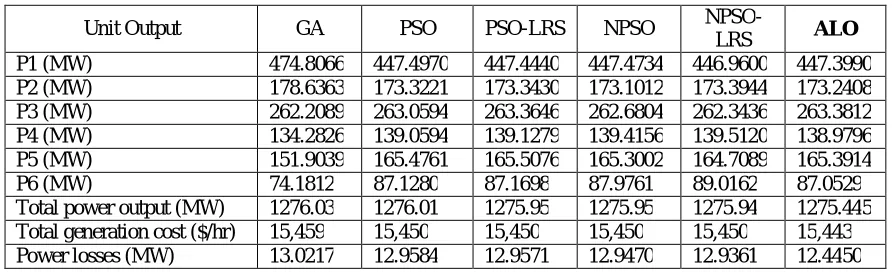
The obtained results for the 6-unit system using the ALO algorithms are given in Table 3 and the results are compared with other methods reported in literature, including GA, PSO, PSO-LRS, NPSO, and NPSO-LRS [18]. It can be observed that the proposed algorithm can get total generation cost of 15,443 $/hr and power losses of 12.4450 MW, which is the best solution among all the methods. Note that the outputs of the generators are all within the generator’s permissible output limit.

Table 3 Comparison of the best results of each methods (PD = 1263 MW)

Unit Output GA PSO PSO-LRS NPSO

NPSO-LRS ALO

P1 (MW) 474.8066 447.4970 447.4440 447.4734 446.9600 447.3990 P2 (MW) 178.6363 173.3221 173.3430 173.1012 173.3944 173.2408 P3 (MW) 262.2089 263.0594 263.3646 262.6804 262.3436 263.3812 P4 (MW) 134.2826 139.0594 139.1279 139.4156 139.5120 138.9796 P5 (MW) 151.9039 165.4761 165.5076 165.3002 164.7089 165.3914

P6 (MW) 74.1812 87.1280 87.1698 87.9761 89.0162 87.0529

Total power output (MW) 1276.03 1276.01 1275.95 1275.95 1275.94 1275.445 Total generation cost ($/hr) 15,459 15,450 15,450 15,450 15,450 15,443 Power losses (MW) 13.0217 12.9584 12.9571 12.9470 12.9361 12.4450

Test Case 2: 40-unit system

This system consisting of 40 generating units and the input data for 40-generator system is given in Table 4 [10]. The total demand is set to 10,500 MW.

results show that the proposed methods are feasible and indeed capable of acquiring better solution. The optimal dispatches of the generators are listed in Table 5. Also note that all generators’ outputs are within its permissible limits.

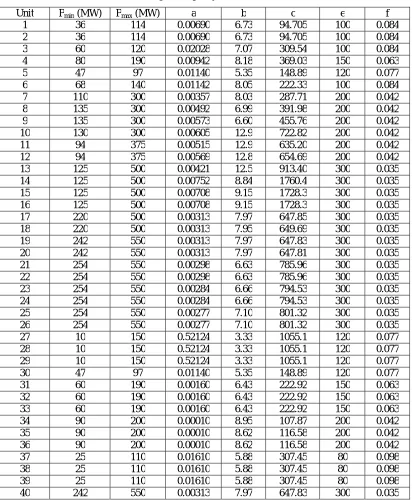
Table 4 Generating unit capacity and coefficients (40-units)

Unit Pmin (MW) Pmax (MW) a b c e f

1 36 114 0.00690 6.73 94.705 100 0.084

2 36 114 0.00690 6.73 94.705 100 0.084

3 60 120 0.02028 7.07 309.54 100 0.084

4 80 190 0.00942 8.18 369.03 150 0.063

5 47 97 0.01140 5.35 148.89 120 0.077

6 68 140 0.01142 8.05 222.33 100 0.084

7 110 300 0.00357 8.03 287.71 200 0.042

8 135 300 0.00492 6.99 391.98 200 0.042

9 135 300 0.00573 6.60 455.76 200 0.042

10 130 300 0.00605 12.9 722.82 200 0.042

11 94 375 0.00515 12.9 635.20 200 0.042

12 94 375 0.00569 12.8 654.69 200 0.042

13 125 500 0.00421 12.5 913.40 300 0.035

14 125 500 0.00752 8.84 1760.4 300 0.035

15 125 500 0.00708 9.15 1728.3 300 0.035

16 125 500 0.00708 9.15 1728.3 300 0.035

17 220 500 0.00313 7.97 647.85 300 0.035

18 220 500 0.00313 7.95 649.69 300 0.035

19 242 550 0.00313 7.97 647.83 300 0.035

20 242 550 0.00313 7.97 647.81 300 0.035

21 254 550 0.00298 6.63 785.96 300 0.035

22 254 550 0.00298 6.63 785.96 300 0.035

23 254 550 0.00284 6.66 794.53 300 0.035

24 254 550 0.00284 6.66 794.53 300 0.035

25 254 550 0.00277 7.10 801.32 300 0.035

26 254 550 0.00277 7.10 801.32 300 0.035

27 10 150 0.52124 3.33 1055.1 120 0.077

28 10 150 0.52124 3.33 1055.1 120 0.077

29 10 150 0.52124 3.33 1055.1 120 0.077

30 47 97 0.01140 5.35 148.89 120 0.077

31 60 190 0.00160 6.43 222.92 150 0.063

32 60 190 0.00160 6.43 222.92 150 0.063

33 60 190 0.00160 6.43 222.92 150 0.063

34 90 200 0.00010 8.95 107.87 200 0.042

35 90 200 0.00010 8.62 116.58 200 0.042

36 90 200 0.00010 8.62 116.58 200 0.042

37 25 110 0.01610 5.88 307.45 80 0.098

38 25 110 0.01610 5.88 307.45 80 0.098

39 25 110 0.01610 5.88 307.45 80 0.098

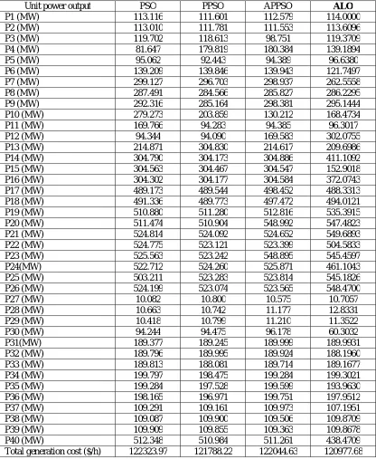
Table 5 Comparison of the best results of each methods (PD = 10,500 MW)

Unit power output PSO PPSO APPSO ALO

P1 (MW) 113.116 111.601 112.579 114.0000

P2 (MW) 113.010 111.781 111.553 113.6096

P3 (MW) 119.702 118.613 98.751 119.3709

P4 (MW) 81.647 179.819 180.384 139.1894

P5 (MW) 95.062 92.443 94.389 96.6380

P6 (MW) 139.209 139.846 139.943 121.7497

P7 (MW) 299.127 296.703 298.937 262.5558

P8 (MW) 287.491 284.566 285.827 286.2295

P9 (MW) 292.316 285.164 298.381 295.1444

P10 (MW) 279.273 203.859 130.212 168.4734

P11 (MW) 169.766 94.283 94.385 96.3017

P12 (MW) 94.344 94.090 169.583 302.0755

P13 (MW) 214.871 304.830 214.617 209.6986

P14 (MW) 304.790 304.173 304.886 411.1092

P15 (MW) 304.563 304.467 304.547 152.9018

P16 (MW) 304.302 304.177 304.584 372.0743

P17 (MW) 489.173 489.544 498.452 488.3313

P18 (MW) 491.336 489.773 497.472 494.0121

P19 (MW) 510.880 511.280 512.816 535.3915

P20 (MW) 511.474 510.904 548.992 547.4823

P21 (MW) 524.814 524.092 524.652 549.6893

P22 (MW) 524.775 523.121 523.399 504.5833

P23 (MW) 525.563 523.242 548.895 545.4597

P24(MW) 522.712 524.260 525.871 461.1043

P25 (MW) 503.211 523.283 523.814 545.1826

P26 (MW) 524.199 523.074 523.565 548.4700

P27 (MW) 10.082 10.800 10.575 10.7057

P28 (MW) 10.663 10.742 11.177 12.8331

P29 (MW) 10.418 10.799 11.210 11.3522

P30 (MW) 94.244 94.475 96.178 60.3032

P31(MW) 189.377 189.245 189.999 189.9931

P32 (MW) 189.796 189.995 189.924 188.1960

P33 (MW) 189.813 188.081 189.714 189.1677

P34 (MW) 199.797 198.475 199.284 199.3021

P35 (MW) 199.284 197.528 199.599 193.9630

P36 (MW) 198.165 196.971 199.751 197.9512

P37 (MW) 109.291 109.161 109.973 107.1951

P38 (MW) 109.087 109.900 109.506 109.8709

P39 (MW) 109.909 109.855 109.363 109.8678

P40 (MW) 512.348 510.984 511.261 438.4709

Total generation cost ($/h) 122323.97 121788.22 122044.63 120977.68

V. CONCLUSION

REFERENCES

[1] A. J. Wood, B. F. Wollenberg, Power Generation, Operation, and Control, 2nd _{ed., John Wiley and Sons, New York, 1996.}

[2] Z. X. Liang, J. D. Glover, “A zoom feature for a dynamic programming solution to economic dispatch including transmission losses”, IEEE Transactions on Power Systems, vol. 7, no. 2, pp. 544-550, May 1992.

[3] P. H. Chen, H. C. Chang, “Large-scale economic dispatch by genetic algorithm”, IEEE Transactions on Power Systems, vol. 10, no. 4, pp. 1919-1926, 1995.

[4] C. L. Chiang, “Improved genetic algorithm for power economic dispatch of units with valve-point effects and multiple fuels”, IEEE Transactions on Power Systems, vol. 20, no. 4, pp. 1690-1699, 2005.

[5] W. M. Lin, F. S. Cheng, M. T. Tsay, “An improved tabu search for economic dispatch with multiple minima”, IEEE Transactions on Power Systems, vol. 17, no. 1, pp. 108-112, 2002.

[6] K. P. Wong, C. C. Fung, “Simulated annealing based economic dispatch algorithm”, Proc. Inst. Elect. Eng. C, vol. 140, no. 6, pp. 509-515, 1993.

[7] J. H. Park, Y. S. Kim, I. K. Eom, K. Y. Lee, “Economic load dispatch for piecewise quadratic cost function using Hopfield neural network”, IEEE Transactions on Power Systems, vol. 8, no. 3, pp. 1030-1038, 1993.

[8] K. Y. Lee, A. Sode-Yome, J. H. Park, “Adaptive Hopfield neural network for economic load dispatch”, IEEE Transactions on Power Systems, vol. 13, no. 2, pp. 519-526, 1998.

[9] T. Jayabarathi, G. Sadasivam, “Evolutionary programming-based economic dispatch for units with multiple fuel options”, European Trans. Elect. Power, vol. 10, no. 3, pp. 167-170, 2000.

[10] N. Sinha, R. Chakrabarti, P. K. Chattopadhyay, “Evolutionary programming techniques for economic load dispatch”, IEEE Transactions on Evolutionary Computation, vol. 7, no. 1, pp. 83-94, 2003.

[11] H. T. Yang, P. C. Yang, C. L. Huang, “Evolutionary programming based economic dispatch for units with non-smooth fuel cost functions”, IEEE Transactions on Power Systems, vol. 11, no. 1, pp. 112-118, 1996.

[12] M. Vanitha, K. Thanushkodi, “An effective biogeography based optimization algorithm to solve economic load dispatch problem”, Journal of Computer Science, vol. 8, no. 9, pp. 1482-1486, 2012.

[13] Hardiansyah, “Artificial bee colony algorithm for economic load dispatch problem”, IAES International Journal of Artificial Intelligence, vol. 2, no. 2, pp. 90-98, 2013.

[14] Z. L. Gaing, “Particle swarm optimization to solving the economic dispatch considering the generator constraints”, IEEE Transactions on Power Systems, vol. 18, no. 3, pp. 1187-1195, 2003.

[15] J. B. Park, K. S. Lee, J. R. Shin, K. Y. Lee, “A particle swarm optimization for economic dispatch with nonsmooth cost functions”, IEEE Transactions on Power Systems, vol. 20, no. 1, pp. 34-42, 2005.

[16] J. B. Park, Y. W. Jeong, J. R. Shin, K. Y. Lee, J. H. Kim, “A hybrid particle swarm optimization employing crossover operation for economic dispatch problems with valve-point effects”, Engineering Intelligent Systems for Electrical Engineering and Communications, vol. 15, no. 2, pp. 29-34, 2007.

[17] Shi Yao Lim, Mohammad Montakhab, Hassan Nouri, “Economic dispatch of power system using particle swarm optimization with constriction factor”, International Journal of Innovations in Energy Systems and Power, vol. 4, no. 2, pp. 29-34, 2009.

[18] A. I. Selvakumar, K. Thanushkodi, “A new particle swarm optimization solution to nonconvex economic dispatch problems”, IEEE Transactions on Power Systems, vol. 22, no. 1, pp. 42–51, Feb. 2007.

[19] S. Mirjalili, “The Ant Lion Optimizer”. Advanced in Engineering, Software, vol. 83, pp. 80-98, 2015.