Automatic Generation Control of Three
Area Power System with Artificial Intelligent
Controllers
Sirisha Annam1, Dr.K.Radha Rani 2, J.Srinu Naick3
PG Scholar, Dept. of EEE, RVR &JC College of Engineering, Andhra Pradesh, India1
Professor, Dept. of EEE, RVR &JC College of Engineering, Andhra Pradesh, India 2
Associate Professor, Dept. of EEE, Sai Tirumala NVR Engineering College, Andhra Pradesh, India3
ABSTRACT: This paper presents decentralized control scheme for Load Frequency Control in a multi-area Power System by appreciating the performance of the methods in a single area power system. A number of modern control techniques are adopted to implement a reliable stabilizing controller. A serious attempt has been undertaken aiming at investigating the load frequency control problem in a power system consisting of three power generation unit and load units. In this paper, change in frequency was observed for the system without control; with PI and PID. Proportional Integral controller approach of automatic generation control along with fuzzy controller are also been examined. PI and PID based AGC have been used for all optimization purposes. The response of frequency change in individual area due to PI and PID with fuzzy based AGC controllers have been compared with the system without control.
KEYWORDS: Load frequency controller, Proportional Integral (PI) controller, Proportional Integral Derivative (PID) controller, Automatic Generation Control (AGC), and Multi-Area Power System.
I.INTRODUCTION
Power systems are very large and complex electrical networks consisting of generation networks, transmission networks and distribution networks along with loads which are being distributed throughout the network over a large geographical area. In the power system, the system load keeps changing from time to time according to the needs of the consumers. So properly designed controllers are required for the regulation of the system variations in order to maintain the stability of the power system as well as guarantee its reliable operation.
The rapid growth of the industries has further lead to the increased complexity of the power system. Frequency is greatly depends on active power and the voltage greatly depends on the reactive power. So the control difficulty in the power system may be divided into two parts .One is related to the control of the active power along with the frequency whereas the other is related to the reactive power along with the regulation of voltage. The active power control and the frequency control are generally known as the Automatic Load Frequency Control (ALFC) [1].Basically the Automatic Load Frequency Control (ALFC) deals with the regulation of the real power output of the generator and its frequency (speed). Automatic Generation Control (AGC) is associate integral a part of Energy Management System [2-6]. This paper deals with the automatic generation control of interconnected multi area grid network.
II.DESIGN MODEL FOR AGC
2.1. Single Area System:
by another control loop, which is called supplementary loop. Due to change in load there is change in the steady state
frequency (∆ω) so we need another loop apart from primary loop to convey the frequency to the initial value, before the
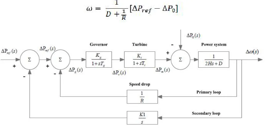
load disturbance occurs. The integral controller which is responsible in making the frequency deviation zero is put in the secondary loop as shown in Fig 1.
Therefore the signal from ∆ω(s) is being fed back all the way through an integrator block (1/s) to regulate ∆Pref to get the frequency value to steady state. Thus ∆ω(s) = 0. Thus integral action is responsible for automatic
adjustment of ∆Pref making ∆ω = 0. So this act is known as Automatic Load Frequency Control transfer function with
integral group is shown below by representing it in the form of equation.
Figure 1: The block diagram representation of single area AGC
2.2. Two Area System:
Two area interconnected system which is joined by means of tie-lines for the flow of tie-line power is given in Fig 2. Let the additional input be ∆P12, ∆P01 be the load change in area1 and the respective frequencies of the two areas
be
∆ω = ∆ω1 = ∆ω2
Let X12 be the reactance of the tie line, then power delivered from area 1 to area 2 is
When X12 = X1 + Xtie + X2 and δ12 = δ1 – δ2
The tie-line power deviation:
∆P12 = Ps (∆δ1 - ∆δ2)
Let ∆ω = ∆ω1 = ∆ω2.
For Area 1,
∆Pm1 -∆P12 - ∆P01 = ∆ωD1
∆Pm1 = - ∆Pm2 = ∆P12 = ∆ωD2
For Area 2,
∆Pm1 = -∆ω/R1
∆Pm2 = -∆ω/R2
Figure 2: Model of two area system without using secondary loop or using only primary loop control
Thus rise in load in area 1 reduces the frequency of both the areas and leads to the flow of tie-line power. If
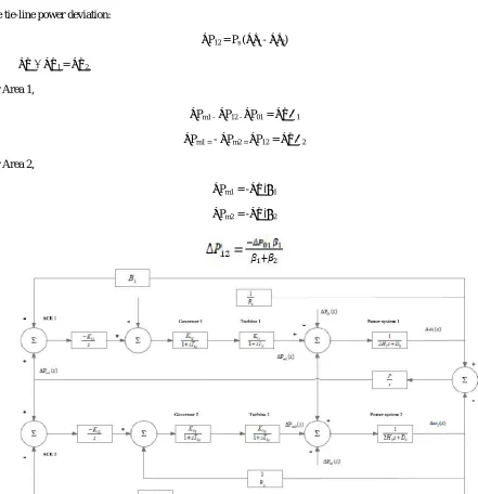
Figure 3: Model of Two Area System with PI Controller
The secondary control basically restores balance linking all area load generation which is possible by maintaining the frequency at scheduled value and is shown in Figure 3. Suppose there is a variation in load in area 1 then the secondary control is in area 1 and not in area 2 so area control error (ACE) is being brought to use. The ACE constituting two areas is represented as follows:
In case of area 1:
ACE1 = ∆P12 + ᵝ1 ∆ω
In case of area 2:
ACE2 = ∆P21 + ᵝ2 ∆ω
For an entire load change of ∆PD the steady state frequency deviation in two areas is
There can be one ALFC for every control area in an interrelated multi area system. ACEs are the actuating signals that stimulate modifications in reference power set points such that ∆P12 and ∆ω becomes zero as soon as
steady-state is attained.
Each area ACE is a combination of frequency as well as tie-line error.
ACEi = Σnj = ∆Pij + Ki∆ω
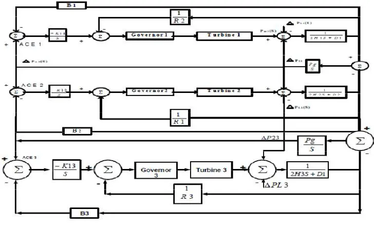
2.3 Three – Area System
coherent. This is referred to as control area. The various control areas are generally interconnected using transmission lines called “tie lines” which allow the flow of active power from one area to another when required.
Figure 3: Three – Area System
2.3.1 Three – Area System without ALFC:
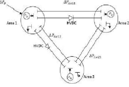
Currently system became too complex with addition of more utilities, which may leads to a condition where supply and demand has got a wide gap. Due to heavy load condition in tie-lines by electric power exchange results in poor damping which may leads to inter-area oscillation. Since the loading conditions are unpredictable, this makes the operation more complex. It has been a topic of concern, right from the beginning of interconnected power system operation. The block diagram of interconnected generating system is shown in fig 4. These three generating areas are interconnected by tie lines.
Figure 4: Three-area power generation system
2.3.2 Three-Area with ALFC:
than others would reduce its generation, while others raised, both attempting to force frequency (as they each measured it to the scheduled value.
Figure 5: AGC for three-area operation
The control in three area system is like the two area system and is shown in above Fig 5. The integral control loop which is used in the single area system and two area system can also be related to the three area systems. Due to change
in load there is change in the steady state frequency (∆ω) so we need another loop apart from primary loop to make the
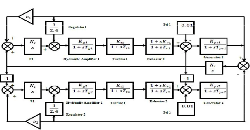
Figure 6: Model of three area system
Change in frequency for the three areas is as follows:
Furthermore, the coordination packet is assumed to be small enough to be transmitted within slot duration. Instead of a common control channel, FHS provides a diversity to be able to find a vacant channel that can be used to transmit and receive the coordination packet. If a hop of FHS, i.e., a channel, is used by the primary system, the other hops of FHS can be tried to be used to coordinate. This can allow the nodes to use K channels to coordinate with each other rather than a single control channel. Whenever any two nodes are within their communication radius, they are assumed to meet with each other and they are called as contacted. In order to announce its existence, each node periodically broadcasts a beacon message to its contacts using FHS. Whenever a hop of FHS, i.e., a channel, is vacant, each node is assumed to receive the beacon messages from their contacts that are transiently in its communication radius.
III. CONVENTIONAL CONTROLLERS
predict target motion. Fuzzy Logic could be used as it has proven to be more efficient than PI controllers and depends on human experience and intuition.
3.1 Proportional term:
The proportional term (sometimes called gain) makes a change to the output that is proportional to the current error value. The proportional response can be adjusted by multiplying the error by a constant Kp, called the proportional gain.
The proportional term is given by
Pout = Kp e(t)
Where,
Pout = Proportional term of output
Kp = Proportional gain, a tuning parameter E = Error = Set value - Actual value T = Instantaneous time in sec. 3.2 Integral term:
The contribution from the integral term (sometimes called reset) is proportional to both the magnitude of the error and the duration of the error. Summing the instantaneous error over time (integrating the error) gives the accumulated offset that should have been corrected previously. The accumulated error is then multiplied by the integral gain and added to the controller output. The magnitude of the contribution of the integral term to the overall control action is determined by the integral gain, Ki.
The integral term is given by ,
Where,
Iout = Integral term of output
Ki = Integral gain, a tuning parameter e = Error = Set Value- Actual Value t = instantaneous time
τ = a dummy integration variable 3.3 Conventional PI Controller:
This controller is one of the most popular in industry. The proportional gain provides stability and high frequency response. The integral term insures that the average error is driven to zero. Advantages of PI include that only two gains must be tuned, that there is no long-term error, and that the method normally provides highly responsive systems. The predominant weakness is that PI controllers often produce excessive overshoot to a step command. The PI controller is characterized by the transfer function
The PI controller is a lag compensator. It possesses a zero at s = -1/Ti and a pole at s = 0. Thus, the characteristic of the PI controller is infinite gain at zero frequency. This improves the steady-state characteristics. However, inclusion of the PI control action in the system increases the type number of the compensated system by 1, and this causes the compensated system to be less stable or even makes the system unstable. Therefore, the values of Kp and Ti must be chosen carefully to ensure a proper transient response. By properly designing the PI controller, it is possible to make the transient response to a step input exhibit relatively small or no overshoot. The speed of response, however, becomes much slower.
3.4 Conventional PID controllers:
A Conventional PID controller is most widely used in industry due to ease in design and inexpensive cost. The PID
formulas are simple and can be easily adopted to corresponding to different controlled plants but it can‟t yield a good
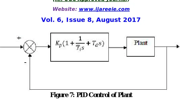
Figure 7: PID Control of Plant
PID is a lag-lead compensator. PI control action and PD control action occur in different frequency regions. The PI control action occurs at the low-frequency region and PD control action occurs at the high- frequency region. The PID control may be used when the system requires improvements in both transient and steady-state performances.
Figure7 shows a PID controller of a plant. If a mathematical model of the plant can be derived, then it is possible to apply various design techniques for determining parameters of the controller that will meet the transient and steady-state specifications of the closed-loop system. However, if the plant is so complicated that its mathematical model cannot be easily obtained, then an analytical approach to the design of a PID controller is not possible. Then we must resort to experimental approaches to the tuning of PID controllers. The process of selecting the controller parameters to meet given performance specifications is known as controller tuning. Ziegler and Nichols suggested rules for tuning PID controllers (meaning to set values Kp, Td and Ti) based on experimental step responses or based on the value of Kp, that results in marginal stability when only proportional control action is used. Such rules suggest a set of values of Kp, Td and Ti that will give a stable operation of the system. However, the resulting system may exhibit a large maximum overshoot in the step response, which is unacceptable. In such a case we need series of fine tunings until an acceptable result is obtained. In fact, the Ziegler-Nichols tuning rules give an educated guess for the parameter values and provide a starting point for fine tuning, rather than giving the final settings for Kp, Ti and Td in a single shot. Because of the complex tuning in PID controller, in this work the tuning is done by hit and trial approach.
Usually the PID controller is a fixed parametric controller and the power system is dynamic and its configuration changes as its expansion takes place. Hence, fixed parametric PI or PID controllers are unable to give their best responses. To cope up with this complex, dynamic and fuzzy situations, fuzzy logic was proposed in literature by many researchers.
3.5 Fuzzy logic Controller:
Fuzzy logic was initiated in 1965 by Lotfi A. Zadeh, professor in Department of Computer Science at the University of California in Berkeley. Fuzzy set theory and fuzzy logic establish the rules of a nonlinear mapping. The use of fuzzy sets provides a basis for a systematic ways for the application of uncertain and indefinite models. Fuzzy control is based on a logical system called fuzzy logic which is much closer in spirit to human thinking and natural language than classical logical systems. Now a days fuzzy logic is used in almost all sectors of industry and science.
The idea behind the Fuzzy Logic Controller (FLC) is to fuzzify the controller inputs, and then infer the proper fuzzy control decision based on defined rules. Fuzzy knowledge based system is shown in Figure 7. The FLC output is then produced by defuzzifying this inferred fuzzy control decision. Thus, the FLC processes contain following main components:
Fuzzification
Rules Definition
Inference Engine
Figure 8: Fuzzy knowledge Base System
IV. RESULT AND DISCUSSION
4.1 Single area System by Using Secondary loop:
In Figure 8 , an integral controller by means of a gain i.e. Ki is used to regulate the signal of speed reference i.e. ∆Pref .
so that ∆fs proceeds to zero . Fig. shows the variation in frequency output with time. The drift in frequency has been
brought to zero because of the integral loop. We have taken the values of the different parameters as shown in below figure 9 for modeling the simulink model and its successful operation to obtain the desired results.
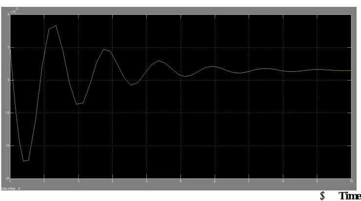
Time
Figure 10: Change in frequency vs. time for single area system by using secondary loop
4.2 Two Area System by Using Secondary loop:
Two area systems by using secondary loop are shown in fig 10 . The secondary loop is responsible for the minimization of drifts in frequency to zero as shown in Fig. By changing the secondary loop gain we can see the variation in the system dynamic response characteristics through tie line power as given away in Fig 11 . We have taken the values of the different parameters as shown in below for modeling the simulink model and its successful operation to obtain the desired results.
4.3 Three-Area System by Using Secondary loop: 4.3.1 Three-Area System without Controller:
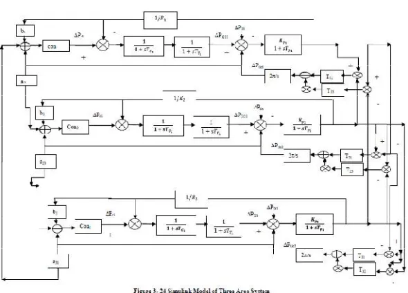
The model for the three area system including the secondary control is given in below Fig 12 . The results of the variation in frequency with respect to time are being shown in Fig 13.
The system operates in a similar way to that of the two area system, taking into consideration the changes in the load. We have taken the values of the different parameters as shown in below for modeling the simulink model and its successful operation to obtain the desired results.
Figure 12: Frequency deviation vs. time for two area by using secondary loop
Figure 14: Frequency deviation vs. time for three-area system without Controller
4.3.2 Three-Area System with PI Controller:
Figure 16: Frequency deviation vs. time for three-area system with PI Controller
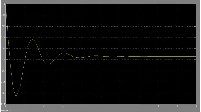
4.3.3. Three-area LFC with PID Controller:
Figure 18: Frequency deviation vs. time of 3-area with PID Controller
4.3.4. Three-area LFC PID with Fuzzy Controller
Figure 20: Frequency deviation vs. time of Three-area LFC PID with Fuzzy Controller
V.CONCLUSION
Change in system frequency is one of the most serious issues in power system as it can cause serious threat to the complete system stability. Load changes are very much common in the power system and this change in load causes the frequency to swing. Control measures have to be taken to control the swing of frequency of the system. Without controller, the change in frequency persists for longer time. Conventional PI controller can be adopted to control the swing but still the swing is found to be sustained for longer time period. Fuzzy controller to control the change in frequency effectively damps the oscillations in system frequency. The comparative analysis of the settling time of frequency in the system without controller, with PI control, PID and PID with Fuzzy controller was explained along with the results. Frequency variations in individual load frequency areas were shown along with their tie-line frequency result of three-area system. From the simulation results, finally it will conclude that the PID with fuzzy controller is better.
REFERENCES
[1]. M.R.I. Sheikh1, R. Takahashi, and J. Tamura “Multi-Area Frequency and Tie-Line Power Flow Control by Coordinated AGC with TCPS” IEEE 6th International Conference on Electrical and Computer Engineering.
[2]. A.Demiroren, “Application of a Self-Tuning to Automatic Generation Control in Power System Including SMES Units”, ETEP, Vol. 12, No. 2, pp. 101-109, March/April 2002.
[3]. Bengiamin, N. N.; Chan, W. C., “Variable Structure Control of Electric Power Generation”, IEEE Trans. on PAS, 101 (1982), 376– 380. [4]. Al-Hamouz, Z. M.; Al-Duwaish, H. N., “A New Load Frequency Variable Structure Controller Using Genetic Algorithms”, Electric Power Systems Research 55 No. 1 (2000), 1–6.
[5]. Jiang, H.; Cai, H.; Dorsey, F.; QU, Z., “Toward a Globally Robust Decentralized Control for Large-Scale Power Systems”, IEEE Trans. on Control System Technology 5 No.3, (1997), 309–319.