ABSTRACT
CHEN, ZHENGZHANG. Discovery of Informative and Predictive Patterns in Dynamic Networks of Complex Systems. (Under the direction of Prof. Nagiza F. Samatova.)
A latent behavior of a dynamic physical system, such as a biological cell or an atmospheric-ocean system is inherently complex. This complexity often arises from the selective, high-dimensional, and nonlinear interconnections of functionally diverse system components to pro-duce coherent behavior. Data-driven prediction or forecast of the system’s behavioral states such as those resulting in land-hitting hurricanes, and discovery of state–determining compo-nents and their cross-talks are challenging. The scarcity and complexity of the available data limit the applicability of the existing machine learning methods to deal with such underdeter-mined, or unconstrained problems. This dissertation addresses these challenges through the following theories and advanced algorithms:
(1) System Phase-related Interplaying Components Enumerator (SPICE) that iteratively enumerates statistically significant components that are hypothesized (1) to play an important role in defining the specificity of the target system’s state(s) or phrases; (2) to exhibit a func-tionally coherent behavior, namely, act in a coordinated manner to perform the state-specific function; and (3) to improve the predictive skill of the system’s states when used collectively in the ensemble of predictive models. When tested on the three important biological problems— identification of biohydrogen production, motility, and of cancer-related system components— SPICEdemonstrated the superior performance in terms of various skill and robustness metrics, including more than 10% accuracy increase on eight real-world data sets.
(2) The network-based community dynamics theory and scalable algorithm to uncover and characterize the community-based dynamics in system networks with multi-functional com-munities. The underlying theory for representative-based detection of all possible dynamic communities—grown, shrunken, merged, split, born, or vanished—ensures the scalability and practical applicability of the algorithm. The runtime speedup of 11–46 over the baseline al-gorithm is observed. Significant and informative community-based dynamics are discovered in the Food Web and Enron networks.
Discovery of Informative and Predictive Patterns in Dynamic Networks of Complex Systems
by
Zhengzhang Chen
A dissertation submitted to the Graduate Faculty of North Carolina State University
in partial fulfillment of the requirements for the Degree of
Doctor of Philosophy
Computer Science
Raleigh, North Carolina 2012
APPROVED BY:
Prof. Steffen Heber Prof. Anatoli V. Melechko
BIOGRAPHY
Zhengzhang Chen received a Bachelor of Science (BS) in Mathematics (with Honors) from Central South University, China in Summer 2005, with a minor in Business Administration. He was recommended to the master program of Computer Science Department at Beihang University exempting from the Chinese National Graduate Entrance Test. He completed his Master of Engineering in Computer Science from Beihang University, China in 01/2008. He was enrolled in North Carolina State University’s Ph.D. program in 8/2008 with a Teaching Assistantship. From Fall 2008 to Fall 2009, he served as a Teaching Assistant for Design and Analysis of Algorithms and C and Software Tools. He was nominated by Dr. Steffen Heber for an Outstanding Teaching Assistant award in Fall 2009. In 2010, he began working under Dr. Nagiza F. Samatova as a Research Assistant in data mining and machine learning. He passed the Written Qualifier in Spring 2010, and completed the Oral Examination in Summer 2011.
Supporting Publications (Chronologically Ordered)
1. Z. Chen, K. Padmanabhan, A. Rocha, Y. Shpanskaya, J. R. Mihelcic, K. Scott, and N. F. Samatova, “SPICE: Discovery of Phenotype-Determining Component Interplays,” BMC Systems Biology, vol. 6(1), pp. 40, PMID: 22583800, 2012.
2. Z. Chen, W. Hendrix, G. Han, I. K. Tetteh, A. Choudhary, F. H. M. Semazzi, and N. F. Samatova, “Detecting Predictive and Physically Interpretable Communities in Contrast Groups of Networks: Application to Adverse Spatio-Temporal Extremes,” Data Mining and Knowledge Discovery Journal, 2012 (2nd Revision).
3. K. Padmanabhan, Z. Chen, S. Lakshminarasimhan, S. S. Ramaswamy, and B. T. Richard-son, “Graph-based Anomaly Detection,” Practical Data Mining with R, Book Chapter, 2012 (In Press).
4. I. Tetteh, D. Gonzalez, Z. Chen, N. F. Samatova, and F. H. M. Semazzi, “An Application of a Newly Developed Machine Learning Technique for Predicting Climate-Meningitis Sea-sonal Outlook Over West Africa,”92nd American Meteorological Society Annual Meeting, 2012.
5. Z. Chen, W. Hendrix, and N. F. Samatova, “Community-based Anomaly Detection in Evolutionary Networks,” Journal of Intelligent Information Systems: Integrating Artifi-cial Intelligence and Database Technologies, vol. 39(1), pp. 59–85, 2012.
Event Tracks in Multi-Variate Spatio-Temporal Physical Systems Using Dynamic Network Structures: Application to Hurricane Track Prediction,” The 22nd International Joint Conference on Artificial Intelligence (IJCAI) 2011, pp. 1478–1484, 2011. ∗: Both authors contribute equally.
7. Z. Chen, T. Pansombut, W. Hendrix, D. Gonzalez, F. H. M. Semazzi, A. Choudhary, V. Kumar, A. V. Melechko, and N. F. Samatova, “Forecaster: Forecast Oriented Feature Elimination-based Classification of Adverse Spatio-Temporal Extremes,”NCSU Technical Report, 1840.2/2408, 2011.
8. M. Schmidt, A. Rocha, K. Padmanabhan, Z. Chen, K. Scott, J. R. Mihelcic, and N. F. Samatova, “Efficient Alpha, Beta–Motif Finder for Identification of Phenotype-related Functional Modules,”BMC Bioinformatics, vol. 12, pp. 440, 2011.
9. K. Wilson, A. Rocha, K. Padmanabhan, K. Wang, Z. Chen, Y. Jin, J. R. Mihelcic, and N. F. Samatova, “Detecting Pathway Cross–Talks by Analyzing Conserved Functional Mod-ules across Multiple Phenotype-Expressing Organisms,” IEEE International Conference on Bioinformatics and Biomedicine (BIBM) 2011 pp. 443–449, 2011.
10. Z. Chen, K. Wilson, Y. Jin, W. Hendrix, and N. F. Samatova, “Detecting and Tracking Community Dynamics in Evolutionary Networks,”The 10th IEEE International Confer-ence on Data Mining (ICDM) Workshop on Social Interactions Analysis and Services Providers (SIASP) 2010, pp. 318–327, 2010.
ACKNOWLEDGEMENTS
First and foremost, I would like to express my special appreciation and thanks to my advisor, Prof. Nagiza F. Samatova, for her tremendous support and guidance throughout my gradu-ate career. I would also like to thank my committee members, Profs. Steffen Heber, Anatoli Melechko, and Fredrick H. M. Semazzi for their helpful suggestions and comments.
I would also like to thank the fellow graduate students at NCSU for their support, especially, William Hendrix, Wenbin Chen, Kanchana Padmanabhan, Andrea Rocha, Tatdow Pansombut, Huseyin Sencan, John Jenkins, Isaac K. Tetteh, Matt Schmidt, Doel Gonzalez, Kevin Wilson, Zhenhuan Gong, and Ye Jin.
Additionally, I would like to thank Prof. Mladen Vouk, Prof. David Thuente, Prof. Douglas Reeves, Prof. Carla D. Savage, Prof. Matthias Stallmann, Prof. Kemafor Anyanwu, Prof. Ben Watson, Margery Page, Carol Allen, and the rest of the faculty and staff of the Department of Computer Science at NCSU for their help over the years.
Finally, I would like to thank my parents, my sister, my brothers and the rest of my family for all of their constant support and encouragement.
TABLE OF CONTENTS
List of Tables . . . vii
List of Figures . . . .viii
Chapter 1 Introduction . . . 1
1.1 Discovery of System’s State Determining Component Interplays . . . 3
1.2 Discovery of Community Dynamics in Evolutionary Networks . . . 4
1.3 Discovery of Anomalous Communities in Contrasting Groups of Networks . . . . 4
Chapter 2 Discovery of System’s State Determining Component Interplays . . 6
2.1 Introduction . . . 6
2.2 Related Work . . . 8
2.3 Method . . . 10
2.3.1 Step 1: Identifying Candidate Component Interplays . . . 11
2.3.2 Step 2: Scoring Candidate Component Interplays . . . 14
2.3.3 Step 3: Assessing Statistical Significance . . . 15
2.3.4 Step 4: Iterative “Knock-out” of Component Interplays . . . 15
2.3.5 Step 5: Bringing Component Interplays Altogether . . . 17
2.4 Results . . . 18
2.4.1 State-Specificity Determining Components . . . 18
2.4.2 Topological Connectivity of Components . . . 27
2.4.3 Functional Enrichment of Component Interplays . . . 27
2.4.4 Predictive Skill of System’s States . . . 28
2.5 Conclusion . . . 32
Chapter 3 Discovery of Community Dynamics in Evolutionary Networks . . . 33
3.1 Introduction . . . 33
3.2 Problem Statement . . . 35
3.3 Application of Community Dynamic Detection to Real-world Dynamic Networks 40 3.4 Community Dynamic Detection Algorithm . . . 44
3.4.1 Lemmas and Theorems . . . 45
3.4.2 Decision Rules for Community Dynamic Detection . . . 48
3.4.3 Algorithm Description . . . 49
3.5 Effectiveness of Representative-based Methodology . . . 53
3.6 Related Work . . . 58
3.7 Conclusion . . . 60
Chapter 4 Discovery of Anomalous Communities in Contrasting Groups of Networks . . . 62
4.1 Introduction . . . 62
4.3 Method . . . 68
4.3.1 Step 1: Abstracting the Dynamic System . . . 68
4.3.2 Step 2: Data Preprocessing . . . 70
4.3.3 Step 3: Identifying Phase-related System Components . . . 71
4.3.4 Step 4: Constructing Contrast-based Groups of Networks . . . 73
4.3.5 Step 5: Enumerating (µ, γ)-communities . . . 74
4.3.6 Step 6: Detecting and Tracking Anomalous Communities in Contrasting Groups of Networks . . . 75
4.3.7 Step 7: Building an Ensemble of Classifiers from Anomalous Communities 76 4.4 Experimental Results . . . 78
4.4.1 Data and Tasks . . . 78
4.4.2 State Determining Communities . . . 79
4.4.3 Predictive Skill of System’s States . . . 82
4.5 Discussion . . . 84
4.5.1 Parameter Selection . . . 84
4.5.2 Generalization: Detecting Biologically Relevant Functional Modules through Biological Networks . . . 85
4.5.3 Comparison to the Modularity-based Community Detection . . . 86
4.6 Conclusions . . . 87
Chapter 5 Conclusion and Future Work . . . 89
LIST OF TABLES
Table 2.1 H2-related enzymes detected by different methods . . . 22
Table 2.2 Cancer-related genes found by SPICE . . . 27
Table 2.3 Microarray data sets . . . 28
Table 2.4 Performance comparison on microarray data sets . . . 29
Table 2.5 Performance on two-class data sets . . . 31
Table 2.6 Performance on multi-class data sets . . . 31
Table 2.7 Bootstrapping performance . . . 32
Table 2.8 Accuracy improvement over a single base classifier . . . 32
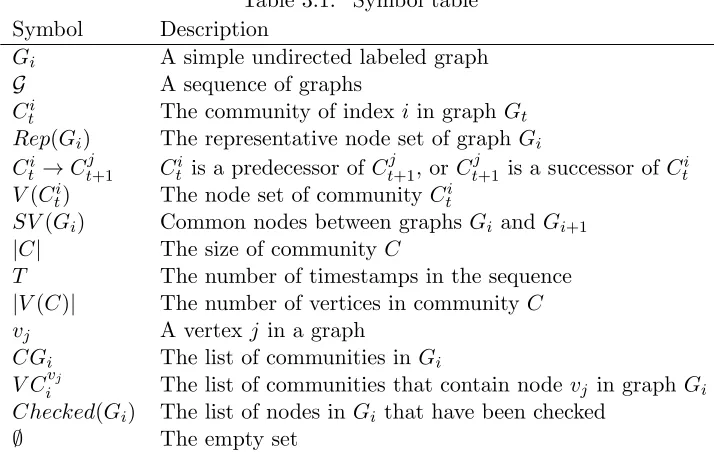
Table 3.1 Symbol table . . . 36
Table 3.2 Food Web communities . . . 40
Table 3.3 Enron email dataset properties . . . 44
Table 3.4 Community dynamics in Enron email dataset . . . 45
Table 3.5 Summary of synthetic datasets . . . 55
Table 3.6 Performance comparison on synthetic data . . . 56
Table 3.7 Effectiveness of graph representatives . . . 57
Table 4.1 Identified climate indices related to hurricane activities . . . 80
Table 4.2 Different modules’ contributions on performance . . . 84
LIST OF FIGURES
Figure 2.1 The overview of SPICE’s key steps. . . 10 Figure 2.2 An illustration of divide-and-conquer strategy for multi-level dimension
reduction. . . 12 Figure 2.3 Fermentation of glucose to generate acetate. Schematic of key metabolic
pathways for hydrogen production inClostridium acetobutylicum. Arrows with larger width indicate a series of reactions. Arrows with narrow width indicate individual reactions. Enzymes: 1, glycolytic enzymes; 2, pyru-vate ferredoxin oxidoreductase (E.C. 1.2.7.1); 3, hydrogenase (E.C.1.12.7.2); 4, phosphotransacetylase (E.C. 2.3.1.8); 5, acetate kinase (E.C. 2.7.2.1). . 20 Figure 2.4 Fermentation of glucose to generate butyrate. Schematic of key
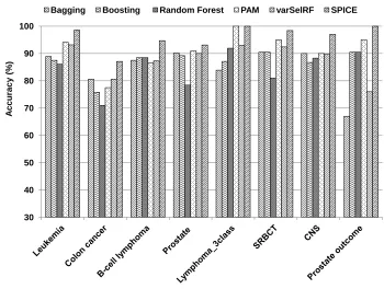
metabol-ic pathways for hydrogen production in Clostridium acetobutylicum. Ar-rows with larger width indicate a series of reactions. ArAr-rows with narrow width indicate individual reactions. Enzymes: 1, glycolytic enzymes; 2, pyruvate ferredoxin oxidoreductase (E.C. 1.2.7.1); 3, hydrogenase (E.C.1.12.7.2); 4, acetyl-CoA acetyltransferase (thiolase) (E.C. 2.3.1.9); 5,β -hydroxybutyryl-CoA dehydrogenase (E.C. 1.1.1.157); 6, crotonase (E.C. 4.2.1.55); 7, butyryl-CoA dehydrogenase (E.C. 1.3.99.2); 8, phosphotransbutyrylase (E.C.2.3.1.19); 9, butyrate kinase (E.C. 2.7.2.7). Abbreviations: Ferre-doxin (Fd); Coenzyme A (CoASH). . . 21 Figure 2.5 Comparison of prediction accuracy of SPICE to other ensemble
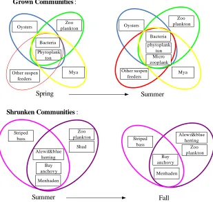
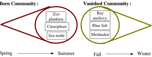
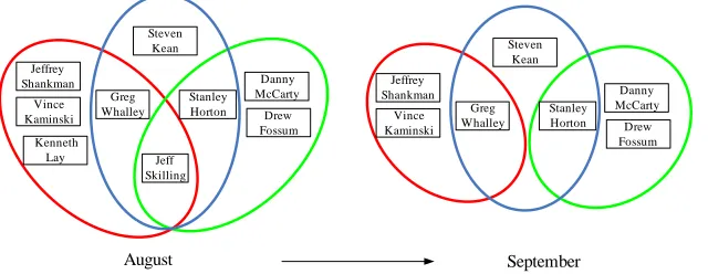
classi-fiers on ten datasets . . . 30 Figure 3.1 Possible types of community dynamics in evolutionary networks . . . 38 Figure 3.2 Example of a grown community and a shrunken community in Food Web. 41 Figure 3.3 Example of a split community and a merged community in Food Web. . 42 Figure 3.4 Example of a born community and a vanished community in Food Web. 42 Figure 3.5 Abnormal communities containing Louise Kitchen in October. . . 43 Figure 3.6 Shrunken communities due to Jeff Skillng resigning as CEO in August. . 43 Figure 3.7 Example for tracking community dynamics using the
non–representative-based method. . . 49 Figure 3.8 Workflow of the community dynamic detection algorithm. . . 50 Figure 3.9 Example for tracking community dynamics using the representative-based
method. Triangles: community representatives; Filled shapes: graph rep-resentatives; Empty shapes: graph-specific vertices; Circles: communities; Dashed lines: predecessor-successor community relationships. . . 51 Figure 3.10 Runtime speedup of the representative-based algorithm over the non–
Figure 3.12 A summary of the various research directions in graph-based anomaly detection. . . 60 Figure 4.1 An example of (µ, γ)-communities. Filled nodes: seed nodes; Empty
nodes: normal nodes. . . 66 Figure 4.2 An example of corresponding communities and conserved communities.
Filled nodes: seed nodes; Empty nodes: normal nodes; Dashed circles: communities. . . 67 Figure 4.3 An example of anomalous communities. C11andC12are conserved
com-munities from the network groupU1, andC21andC22are conserved
com-munities from the network group U2. Filled nodes: seed nodes; Empty
Chapter 1
Introduction
An emerging field in data mining is detecting and analyzing the key features or functional structures governing the behavior of dynamic physical systems across various domains from atmospheric-ocean systems to biological cells [30, 31, 90]. Mining such informative and predic-tive patterns or relationships can help scientists reveal underlying simplicity from complexity [3], develop data-driven approaches for modeling latent system behavior, and complement the typical hypothesis–driven scientific methodologies.
To achieve this goal, researchers often simplify the modeling process of system’s behavior by using some key system components or features. In machine learning, feature selection has been successfully employed to increase the prediction accuracy of classifiers; reduce the computation time of the learning algorithms; increase the robustness of classifiers; and facilitate the interpretability of the derived relationships between features by removing irrelevant and redundant features. The development of feature selection techniques [17, 79, 126, 154] has been an important field in many application domains like climate and biology. For example, in the extreme event prediction, researchers often use the correlation method (e.g., Pearson correlation) to calculate the correlation between each feature and tropical cyclone or rainfall activity, choosing the climate features with the best individual correlations [31, 59].
However, physical dynamic systems are inherently complex, and often operate in multiple phases, described as having similar defining characteristics but whose feedbacks behave in a non-linear fashion [53]. And considering the fact that the number of observational samples to build the prediction models of a real-world system is often significantly fewer than the number of available features, the existing machine learning methods easily become hardly suitable for dealing with such underdetermined, orunconstrained problems.
[45, 155, 123, 20]. Such complex networks model a variety of systems including societies, ecosystems, the Internet, and others [108]. For example, in climate networks [155, 45], the nodes represent the spatial grid points and the edges between pairs of nodes exist depending on the degree of statistical interdependence between the corresponding pairs of anomaly time series taken from the climate data set. Complex networks have enabled hypothesis-driven insights about the intricate interplay between the topology and dynamics of the physical system.
Networks of dynamic systems can be highly clustered [166]. A community, defined as a col-lection of individual objects that interact unusually frequently, is a very common substructure in many networks [55, 45, 155], including social networks, metabolic and protein interaction networks, financial market networks, and even climate networks. For example, in protein inter-action networks, a set of proteins that are strongly related may form a multiprotein complex or perform a function together within a cell [179]. Previous work has been mainly focused on de-tecting community structures in static graphs [55, 34, 129], or dede-tectingconserved communities in evolutionary networks [74, 113, 141].
In spite of the advantages offered by machine learning approaches and graph theoretical approaches to discover some strong patterns in complex systems, there are several challenges that need to be overcome. First, how can we discover the system component interplays in instance-based data? As aforementioned, the system components often form hierarchical func-tional modules (or communities) like protein complexes. Thus, the tradifunc-tional approaches that identify individual components that confer a given system state are likely not optimized to de-tect groups of such interplays between system components. Second, in the networks of dynamic systems, traditional methods can not detect the community dynamics, but only the conserved or stable communities. In networks of biological systems, a small variation in a gene community may indicate an event, such as gene fusion [137], gene fission [137], or gene gain [23]. Final-ly, conventional community detection methods [55, 34, 129, 74, 113, 141] often fail to detect predictive and phase-biased communities that are conserved within one group of networks but undergo statistically significant structural transformation in the other groups of networks. Such anomalous communities could contribute to our understanding of the system’s behavior for a given phase.
1.1
Discovery of System’s State Determining Component
In-terplays
We first approach the problem of enumerating all the groups of cross–talking system components that could be associated with the system state. In dynamic physical systems, it is often a coordinated, not independent, action of several system components determines the system’s state. The main challenge in enumerating of system state-determining component interplays is how to deal with the enormous number of system components (or features) that could easily reach thousands or even hundreds of thousands. Such enormous feature space could easily lead to the problem, coined by Bellman as “the curse of dimensionality” [8], that is, the number of system components (n ≈10,0000s) is significantly larger than the number of observational samples (m ≈ 1000s). Thus, the existing machine learning methods easily become hardly suitable for dealing with such underdetermined, or unconstrained, problems.
We propose an iterative, classification-based approach, calledSPICE(System Phase-related Interplaying Components Enumerator), that comprehensively enumerates the set of feature sub-sets that discriminate between different system states (or classes). Given a set of observations about system components (features) with the corresponding assignment of the system’s state (class), our method measures the importance of feature subsets to discriminate between system states. Despite combinatorial complexity of the problem, our method almost exhaustively ex-ploits feature subsets by focusing on information-theoretic selection process. Our method rests on a hypothesis that if a subset of system components discriminates between system’s func-tional states when considered altogether but not in any subset, then these components most likely form a cross-talking state-determining feature subset. It also places the contribution of an entire feature subset at the core of the analysis as opposed to the approaches that first evaluate the importance of individual features and then filter those that are associated with a particular system’s state. It further filters those feature subsets that are statistically significant and are thus assumed to be relevant to the application domain.
details on SPICE approach appear in Chapter 2. And this work [174] has been published in the Journal of BMC Systems Biology.
1.2
Discovery of Community Dynamics in Evolutionary
Net-works
Although graph-based anomaly detection has been done on exploring three different types of anomalies including anomalous nodes, novelty edges, and abnormal subgraphs, little work has focused on dynamic communities. Communities in the real networks are changing over time. For example, in biological networks, a small variation in a gene-gene association community may represent an event, such as gene fusion [137], gene fission [137], gene gain [23], gene decay [99], or gene duplication [180], that would change the properties of the gene products (e.g., proteins) and, consequently, affect the phenotype of the organism. Detecting community dynamics is essential for a deeper understanding of the development and self-optimization of the system as a whole.
In contrast to the previous work on graph-based anomaly detection and community iden-tification in static graphs or tracking conserved communities in time-varying graphs, we first introduce the concept of community dynamics, and then show that the baseline approach by enumerating all communities in each graph and comparing all pairs of communities between consecutive graphs is infeasible and impractical. We propose an efficient method for detecting and tracking community dynamics in evolutionary networks by introducing graph representa-tives and community representarepresenta-tives to avoid generating redundant communities and limit the search space. When applied to two real-world evolutionary networks, Food Web and Enron Email, significant and informative community-based anomaly dynamics have been detected in both cases.
Further details on our approach, including a theoretical proof that only six types of com-munity dynamics are possible in simple undirected graphs, the decision rules for detecting the dynamic communities, and the completeness of the algorithm, appear in Chapter 3. The re-sults of this work have been published at the IEEE ICDM conference [28] and in Journal of Intelligent Information Systems [27].
1.3
Discovery of Anomalous Communities in Contrasting
Group-s of NetworkGroup-s
can build two different groups of climate networks, with one corresponding to strong TC years, another with corresponding to low TC years. Different groups of networks may exhibit different properties of the community structure. Detecting the anomalous communities in contrasting groups of networks can help us better interpret the physical relevance of the interplaying features determining the system’s phases.
Chapter 2
Discovery of System’s State
Determining Component Interplays
2.1
Introduction
Dynamic physical systems, such as the atmospheric-ocean system or biological cells, are in-herently complex. This complexity arises from the selective and nonlinear interconnections of functionally diverse system components to produce coherent behavior. The key challenge is to reveal underlying simplicity from complexity [3]. Unlike the four Maxwell’s equations describing all the electro-magnetic phenomena from “first principles,” the fundamental rules that quantify the low dimensional behavior of such systems are yet to be discovered.
Complementing approaches based on first principles, where the underlying system model is described by a system of equations, thedata-driven modeling of system behavior is a promising approach. It aims to interrelate data from disparate and noisy experiments and observations to find informative features and link them to formulate fundamental principles governing a complex behavior. This process frequently begins with a comprehensive enumeration of the system “components” (e.g., co-regulated proteins in a cell or climate indices in the atmospheric-ocean system) derived from experimental or observational data. Discovery of putative associations (e.g., teleconnections) between these “components” can then be used to designin silicosystem models (e.g., positive and negative feedbacks, information processing and signal transduction cascades) to better understand real system behavior.
biomass degradation, then enumeration of state-related system components would identify all the proteins involved in degradation of cellulose to sugars, transport of these sugars through the membrane, and their fermentation to ethanol. Likewise, if the target state of the atmospheric-ocean system is the intensity of seasonal hurricane activity (i.e., above normal, normal, or below normal), then enumeration of hurricane activity-related system components would produce a set of putative system’s parameters (e.g., temperature, precipitable water, pressure) associated with particular spatial regions on Earth that likely affect the magnitude of the system’s re-sponse. Similarly, if the system’s state of interest is cancer-prone cells in the human body, then enumeration of cancer-related cellular components would identify all the genes that are likely related to the expression of cancerous cellular phenotype.
The difficulty in enumerating all the state-related system components lies in dealing with the enormous number of system components (or features) that could easily reach thousands or even hundreds of thousands. Such enormous feature space could easily lead to the problem, coined by Bellman as “the curse of dimensionality” [8]. For example, high-resolution ocean-atmospheric models can be defined over the 1.4◦×1.4◦ (latitude, longitude) spatial grid on the globe, several altitude levels, and a few dozen variables.
Likewise, the interaction between two biomolecules, such as protein-protein interactions, can be described through their set of contacting amino acid residues. A possible set of features to describe this interface is enormous due to a number of chemical identities of the contacting residue pairs (210 features from 20 amino acid types), orientation patterns of the contacting residues, and spatial arrangements of 3-5 contacting residues. One needs to select all those features that would provide clear differentiation between the true interfaces and merely feasible associations of two rigid bodies. In addition, hierarchical nature of most biological systems leads to “short- and long-range” interactions between the features. For example, hydrophobic residue pairs could enhance a propensity for other adjacent hydrophobic pairs (“short-range” feature correlation). On the other hand, highly specific residue interactions may be under selective pressure to fit into an overarching architectural motif (such as helix-turn-helix motif), thus contributing to “long-range” feature dependences.
is a need for methods that aim to enumerate all the groups of cross-talking system components that could be associated with the system state. We call this problem the enumeration of system state-determining component interplays.
To address this problem, we propose an iterative, classification-based approach that com-prehensively enumerates the set of feature subsets that discriminate between different system states (or classes). Given a set of observations about system components (features) with the corresponding assignment of the system’s state (class), our method measures the importance of feature subsets to discriminate between system states. Despite combinatorial complexity of the problem, our method almost exhaustively exploits feature subsets by focusing on information-theoretic selection process. Our method rests on a hypothesis that if a subset of system compo-nents discriminates between system’s functional states when considered altogether but not in any subset, then these components most likely form a cross-talking state-determining feature subset. It also places the contribution of an entire feature subset at the core of the analysis as opposed to the approaches that first evaluate the importance of individual features and then filter those that are associated with a particular system’s state. It further filters those feature subsets that are statistically significant and are thus assumed to be relevant to the application domain.
2.2
Related Work
To the best of our knowledge, the proposed problem of enumerating statistically signifi-cant component interplays that are key contributors to the system’s stateshas not been addressed in literature. The problem resembles, yet with quite apparent distinctions, the problems of feature selection, phylogenetic profiling, network alignment, and frequent subgraph mining.
the latter comment. In addition, the runtime for these approaches grows exponentially; even the most efficient ones, such as MULE [92] that enumerates maximal frequent edge sets, took almost 57 days for a set of 98 network instances (details available upon request). While efficient heuristics have been reported [128], they are tailored for specific network types (e.g., metabolic networks).
For the second category, the system is often represented by its set of components (i.e., fea-tures) that are defined over multiple instances (i.e., observations) for each of the finite set of system’s distinct phenotypes. In this case, univariate approaches, such as those that, for the given feature, look for a strong correlation between its profile and the system’s phenotype profile across multiple instances identify a set of putative candidates for component interplays. Dif-ferent correlation measures, such as Pearson correlation, Mutual Information, Student’s t-test, ANOVA, Wilcoxon rank sum, Rank products, and other univariate filter feature selection tech-niques can provide different candidate sets that could be further assessed with set-theoretical approaches to provide either higher specificity (i.e., intersection of sets) or higher sensitivity (i.e., set union).
A particular instance of such a strategy is phylogenetic profiling [136], where different or-ganisms that exhibit various (but finite) phenotypes (e.g., aerobic vs. anaerobic growth) are considered as observations characterized by the the presence or absence of particular genes (or components). The underlying hypothesis behind this approach is that candidate genes are more likely to be present in phenotype-expressing organisms than in phenotype-non-expressing organisms due to an evolutionary pressure to conserve the phenotype-related genes [94]. While simple, fast, and effective [126] in findingindividual components that are likely associated with the system’s phenotype, such methods are quite limited in discovering of the component inter-plays.
System Components
Iterative Decision Tree Component Knock-out
1. Identifying Candidate Component Interplays
System States
2. Scoring Candidate Component Interplays
3. Assessing Statistical Significance
Weighting Scheme 5. Bringing
Component Interplays Altogether Data
4. Iterative “Knock-out” of Component Interplays
Figure 2.1: The overview of SPICE’s key steps.
approaches are very specific to a given classification algorithm.
2.3
Method
2.3.1 Step 1: Identifying Candidate Component Interplays
We hypothesize that if the component is key to defining the system’s state then its value distributions will be separable between the observations from different states. If the separation is strong, then such a component, alone, is likely able to discriminate system states. And almost any method, like entropy-based, would likely succeed in detecting those components. However, with real data sets such a strong separation is less likely. There are different reasons for such an assumption. For example, the evolution of system behavior may induce non-functional changes to the system components. For example, natural mutations in a protein sequence happen all the time; and if much time has passed since the functional divergence occurred, then functional state-preserving mutations must have been compensated by correlated mutations at other positions in the sequence to retain the protein function. As a result, one should strive for discovery of separation signals that while being weaker at the individual component level, they—as a group—should be able to discriminate between system states. Although the validity of this assumption is yet to be verified, numerous studies, such as those on correlated mutations [116, 4, 56, 152], provide indirect evidence in support of such a position. Another reason could be attributed to the noise in the data, for example, due to limited sensitivity of experimental devices. For instance, the chance of observing a strong signal about transient or transmembrane protein interactions from mass spectrometry experiments is low.
Thus, the effective analysis should not only include an individual component with a strong discriminatory signal, but also extend to a group(s) of interplaying components out of a set of thousands of components. This creates a multiplicity of possible combinatorial interplays to search for and excludes a possibility for a brute-force enumeration. Therefore, our goal is to provide a framework for automatic exploration of such combinatorial interplays that could offer both the computational efficiency and the application domain relevance.
In some cases, the domain knowledge may assist with constraining the search space of possible interplays. For example, functionally important amino acid residues, such as substrate binding sites, in a protein are likely located on the surface (i.e., clefts and cavities) of the protein 3-dimensional structure and not in the core. For a more general and domain-independent solution, however, the issue of properly constraining the search space still remains.
clustering (e.g., [68, 69, 72]) or spectral graph partitioning techniques (e.g., [73, 78]).
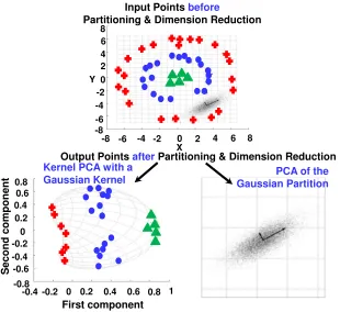
Specifically, the intuition behind our approach stems from the well-known concept of modu-larity, introduced by Hartwellet al. [63], as a generic principle of complex system’s organization and function. These functionally associated modules often combine in a hierarchical manner into larger, less cohesive subsystems, thus revealing yet another the essential design principles of system organization and function–hierarchical modularity [122, 138]. Thus, our method first identifies modules of system components with putatively stronger associations within the mod-ules than between the modmod-ules. This processdivides all system components into modules that likely function together to define what state the system is in. The process furtherconquers each of these modules in order to refine the specificity of the inter-component relationships within the module. Fig. 2.2 shows an illustration of this divide-and-conquer approach to multilevel
dimen-PCA of the Gaussian Partition
-0.2 0.2 0.6 0.8
-0.4 0 0.4 1
-0.6 -0.2 0.2 0.4
-0.8 -0.4 0 0.6 0.8
First component
Se
cond
compon
ent
Output Points after Partitioning & Dimension Reduction
-6 -2 2 4
-8 -4 0 6 8
-6 -2 2 4
-8 -4 0 6 8
X Y
Kernel PCA with a Gaussian Kernel
Input Points before
Partitioning & Dimension Reduction
Figure 2.2: An illustration of divide-and-conquer strategy for multi-level dimension reduction.
together before and after the partition followed by dimension reduction). The standard PCA result performed on the monolithic set is mediocre, i.e., distinguishing the four different groups is impossible using only linear PCA. After partitioning the set, the “appropriate” technique is applied to each partition (bottom): the kernel PCA to the nested ring points (left partition) and the linear PCA to the Gaussian cluster (right partition). As a result, not only is the size of the data reduced for each partition, but also the four groups become distinguishable using only the first principal component.
Unlike the example in Fig. 2.2, in the context of our problem—enumeration of statistically significant and application-relevant component interplays that are key contributors to the sys-tem’s state—we deploy decision tree based procedure for identifying the right partitions of the system’s features and then apply the “appropriate” classification technique to each partition. The reason is that due to highly underdetermined nature of our problem, subsampling of the input data sample could possibly lead to an unreliable inference methodology. Likewise, due to a possibly non-linear interplay between the system’s features, it would be more desirable to divide the system components into “blocks” with possibly stronger interconnects within the blocks and weaker inter-connects between the blocks. This strategy is inspired by the mod-ularity principle of complex systems. Thus, a higher-level supervised separation of the high dimensional feature space into the rectangular shape hyperspaces is achieved via information-theory driven decision boundaries with a subsequent refinement of decision boundaries within the identified subspaces (see Step 2).
We propose a decision tree-based methodology for our feature space partitioning. The features in a decision tree are considered as one feature subset, and each feature is a system component. There are multiple reasons for why we choose decision tree based methodology, including (a) efficiency to process many features (unlike BBNs that are exponential in the number of features), (b) inherently multiclass by nature, and (c) the ability to handle continuous and multi-variate types of features (unlike NNs for which distance metrics are poorly defined for mixed data types), among others. We use the CART-decision tree algorithm [16] to select a set of discriminatory features from the available feature space. Basically, CART builds a decision tree by choosing the locally best discriminatory feature at each split step based on the Gini Index Impurity Function. To avoid overfitting, CART employs backward pruning to build smaller, more general decision trees. CART chooses features in a multivariate fashion, which allows the feature selection process to find a set of discriminatory features instead of considering one feature at a time.
downstream of our analysis pipeline (Step 2 and Step 5). Also, decision boundaries themselves could result in rules that are more interpretable and could provide additional insights to domain scientists on the magnitude of the feature attributes that affect a system’s phenotype. The reason is that not only is it important to know what group of features is contributing to the system’s phenotypic state but to what extent the feature values could change the system’s phenotypic state. For example, if the expression of a particular gene becomes above a certain threshold, then this causes a “knock-out” of a particular metabolic pathway. With decision trees, the full feature space gets partitioned into hypersubspaces by the decision rules of the form of ai ≤ fi ≤ bi. Once this high-level factors contributing to the system’s states are
learned, more complex (e.g., non-linear or conditional) relationships between the components in the group could be learned by more sophisticated classifiers, such as BBNs or kernel SVMs (see Step 2).
2.3.2 Step 2: Scoring Candidate Component Interplays
Candidate system’s components identified in Step 1 are next assessed in terms of theircollective ability to contribute to the system’s states. Basically, the goal is to define a scoring function that could measure how well this group of components (features) discriminates between system phenotypic states. On the one hand, mutual information (MI) for an individual component could be used with its proper generalization to a group of components. However, robust prob-ability estimation—an essential step in MI definition—requires a large sample size, which is often unavailable for underdetermined systems. Moreover, the generalized MI is biased toward the presence of a component in the group with high information content.
2.3.3 Step 3: Assessing Statistical Significance
Given a candidate feature set (Step 1) and its predictive skill score (Step 2), we next assess statistical significance of this score, namely, how likely a similar skill score could be observed at random. Specifically, we want to use the confidence level for the classification accuracy to sift phenotype-specificity determining component groups. It is expected that the statistically significant, highly scored component groups are application-significant. For example, a group of candidate genes could be biologically significant for biohydrogen production or cancer phenotype expression (see Sections 2.4.1).
It is worth observing that, generally, sample instances within the same system phenotype tend to be more similar than those from the other phenotypes. Hence, separation of feature value distributions between the samples from different states will be relatively clearer, and thus classification accuracy—as a measure of feature set’s discriminatory power—can be biased. This implies that standard statistical testing like shuffling the phenotype (class) labels is not acceptable.
Thus, to provide a robust assessment of statistical significance, we measure an empirical p−value of each candidate feature set using the Monte Carlo procedure described in [177]. Specifically, for each feature subset, we randomly sample N feature subsets (N = 1,000) from the entire feature set of the same size as our candidate set, and compute the corresponding accuracies of the classifiers built from these feature sets. Then, we estimate an empirical p−value of the target feature subset as p = (R+ 1)/(N + 1), where N is the total number of random samples (N ∼ 1,000) and R is the number of these samples that produce a test statistic greater than or equal to the value for the target feature subset. This corresponds to the percentile where our target score falls onto within the accuracy distribution forN samples. In our experiments, the selectedp−value meets 95% confidence level. Algorithm 1 presents the detailed pseudo-code for the statistical significance assessment.
2.3.4 Step 4: Iterative “Knock-out” of Component Interplays
Algorithm 1: Statistical significance assessment Input:
F : entire feature set
Fc : candidate set of features
Mc: classifier model learned fromFc
D : entire training data set overF and system phenotypic statesS A : the best performing classifier
α : the required confidence level (e.g., 95%)
N : the number of samples for Monte Carlo estimation Output:
An indicator of the quality ofFc
1 Letc be the training accuracy ofMc 2 Letbe an empty set
3 forN iterationsdo
4 LetFr be a random sample of|Fc|features fromF
5 LetDr be the restriction ofD to the features inFr
6 Train a classifierMr by runningAonDr
7 Calculate the training accuracy ofMr and add it to
8 Calculate ap-value for andc 9 if p-value≤(1−α/100)then 10 returnPASS
11 else
12 returnFAIL
complex system; this redundancy contributes to system’s robustness. Therefore, our task is not simply to identify a single “best” group but, ideally, to enumerate them all.
The combinatorial nature of this task necessitates heuristic approaches. Our strategy is inspired by the way biologists often conduct their mutagenesis studies. Namely, theyknock-out a group of genes (e.g., via gene deletion) and observe themutantsystem’s response. By analogy, our methodology knocks-out the selected candidate feature sets and proceeds with Steps 1-3 on the mutant system in an iterative fashion until some stopping criterion is met (see Line 2 in Algorithm 4). Under this approach, each iteration produces a subset of features out of the current feature set (see Line 4 in Algorithm 4), then removes these features from the set so that they can’t be selected again (see Line 9 in Algorithm 4).
stopping criterion. Line 2–2 in Algorithm 4 summarizes the aforementioned iterative knock-out procedure.
Algorithm 2: SPICE: System’s state determining interplaying components enumer-ator
Input:
F : a set of components (features)
D: a set of training data overF D0: a set of test data overF Y : a set of system states overD A : basic classification algorithms
: (e.g., decision tree, SVM, Na¨ıve Bayes, etc.) Output:
Y0 : predicted states for the test setD0 CIG: identified component-interplay groups
1 CIG← ∅
/* E: save the prediction results of candidate models */
2 E← ∅
3 whilestopping criterion is not metdo
/* Run CART-decision tree to get a candidate component group */
4 A pruned decision treeT ←CART(D,Y)
5 LetFc be a set of all components that belong to the internal nodes ofT
6 DFc ←Extract the data fromD only with the components inFc
7 Prediction skill scorec ←applyingAto DFc 8 LetMc be the classifier model learned fromFc
9 if c meets the statistical significance criterion (see Algorithm 1)then 10 LetDF0
c be the restriction ofD
0 to the features inF
c
11 Predicted system statesYc0 ←ApplyMc toD0Fc
12 AddYc0 toE 13 AddFc toCIG
14 Remove features inFc from F
15 Remove the data over featureFc fromD
16 Predict the class labelsY0 based on a majority vote of the results inE 17 returnY0 andCIG
2.3.5 Step 5: Bringing Component Interplays Altogether
inter-factor relationships could determine the specificity of the system’s state. We then combine these subsystems through the framework of the ensemble methods in order to construct a system-level predictor of system’s behavioral states.
In the last step (Step 5 in Figure 4.4), we need to combine the predictions of all the classifiers that pass statistical significance criterion (Step 3) to come up with the final prediction value. In order for the ensemble to make a prediction, each classifier is given a weighted vote, and the class with the most votes is the prediction of the ensemble (see Line 16 in Algorithm 4). We tested three possible weighting schemes: a simple majority voting scheme, in which every classifier is given equal weight; a training accuracy-based method, in which every classifier is weighted based on its training accuracy; and an internal cross-validation-based voting, in which each classifier is weighted by that model’s cross-validation accuracy on the original training data.
Two of the key characteristics for building a robust classifier ensemble include (a) the diversity among the classifier models in the ensemble [105] and (b) the reasonably high accuracy of the individual members in the ensemble. In our case, the former is ensured due to our feature set knock-out strategy (Step 4) and the latter is guaranteed by a combination of decision-tree based feature enumeration (Step 1), the scoring function (Step 2), and the statistical significance assessment (Step 3) that, in combination, also reduce possible redundancy among the models and thus reduce the possible bias (e.g., due to a significantly large portion of highly similar models). By bringing the enumerated component interplays altogether (Step 5) a good ensemble of classifiers can be achieved (as illustrated in Section 4.4).
2.4
Results
The nature of the proposed methodology,SPICE, suggests that detected component interplays (Steps 1-4) (1) could play an important role in defining the specificity of the system’s state(s); (2) would likely exhibit stronger inter-component relationships within the same group than between the groups and are functionally coherent, namely, act in a coordintaed manner to perform the state-specific function; and (3) collectively, could improve the predictive skill of the system’s states (Step 5).
2.4.1 State-Specificity Determining Components
Groups of Enzymes Associated with Biohydrogen Production
photosyn-thesis [107]. To date, a number of phylogenetically diverse microorganisms have been identified as hydrogen producing. Such organisms include photosynthetic bacteria, nitrogen-fixers, and heterotrophic microorganisms [125]. In order to generate hydrogen, these organisms may rely upon one or more metabolic routes. As such, the biohydrogen production phenotype provides an opportunity to evaluate the capabilities of SPICEto handle a relatively complex phenotype. Identification of phenotype-related components was based on the assumption that if a compo-nent (i.e., a group of enzymes in a metabolic process) is specific to biohydrogen production, then it is likely evolutionarily conserved across H2-producing organisms, and it is absent in
mostH2-non-producing ones.
Our first experiment includes the data about 17 H2-producing and 11 H2-non-producing
microorganisms and compares SPICE’s performance against the two commonly used statis-tical methods: Mutual Information (MI) and Student’s t-test, and one multivariate feature selection approach: SVM recursive feature elimination (SVM-RFE). Among 17 H2-producing
microorganisms, four microorganisms utilize bio-photolysis, five microorganisms utilize light fermentation, and eight microorganisms utilize dark fermentation. 11 microorganisms are list-ed as non-hydrogen producing because they are not associatlist-ed with hydrogen production baslist-ed on literature review, or they lack hydrogenase [76], one of the key enzymes involved in hydrogen production. All microorganisms used in this experiment were verified as completely sequenced using the NCBI database. The input to SPICE is a matrix, with the enzyme EC numbers along the rows, 28 organisms (hydrogen producing and non-producing) along the columns, and the entry in each cell (i, j) is the copy number for enzyme i in organism j. The last row of the matrix includes information about the organism’s ability to express the hydrogen production phenotype.
The mutual information method [81] assesses correlation between the enzyme’s phylogenetic profile and the organism’s H2-production profile across multiple organisms. In addition, it
reports a significance threshold by shuffling the enzyme profile vectors and calculating the mutual information with the organism’s phenotype profile. Only those enzymes, whose mutual information values lie above the confidence cutoff are reported.
The Student’s t-test is another statistical method to identify phenotype related enzymes, where we utilize the enzyme phylogenetic profiles alone to measures statistical bias of enzyme copy numbers in one phenotypic group of organisms vs. the other. The test results are filtered so that only enzymes with thep-value less than 0.05 are considered significant.
Guyon et al.[60] proposed the SVM-RFE algorithm to rank the features (enzymes) based on the value of the decision hyperplane given by the SVM. The features with small ranking scores are removed. The top 240 enzymes (out of 1,229 enzymes) are considered significant.
Glucose
2 CoASH 2 Pyruvate
2 Acetyl-CoA 2 CO2
1
2
3 2 Acetyl-Phosphate 2 Acetate
2 CoASH
2 Pi 2 ADP
2 ATP
4
Fdox
Fdred 2H2
4H+
5
2 ADP
2 ATP
2 NAD+
2 NADH + 2H+ 2H2
Figure 2.3: Fermentation of glucose to generate acetate. Schematic of key metabolic pathways for hydrogen production inClostridium acetobutylicum. Arrows with larger width indicate a se-ries of reactions. Arrows with narrow width indicate individual reactions. Enzymes: 1, glycolyt-ic enzymes; 2, pyruvate ferredoxin oxidoreductase (E.C. 1.2.7.1); 3, hydrogenase (E.C.1.12.7.2); 4, phosphotransacetylase (E.C. 2.3.1.8); 5, acetate kinase (E.C. 2.7.2.1).
fermentation of glucose to acetate (Figure 2.3) and butyrate (Figure 2.4) inClostridium aceto-butylicum. Within this process, glucose is broken down through a series of glycolytic enzymes to generate pyruvate. Pyruvate is then converted to acetyl-CoA through the action of pyru-vate ferredoxin oxidoreductase. During this step, hydrogen gas is produced when pyrupyru-vate is oxidized, thus resulting in the formation of CO2 plus H2. Production of hydrogen via this
route is mediated through two enzymes—pyruvate ferredoxin oxidoreductase and hydrogenase. Acetyl-CoA generated produced from pyruvate can then enter a number of pathways, including the acetate and butyrate formation pathways.
While production of hydrogen occurs predominately during formation of Acetyl-CoA and not in the secondary pathway (e.g., conversion of Acetyl-CoA to acetate), acetate and butyrate fermentation pathways play an important role in the overall yield of hydrogen by microorgan-isms. In metabolic engineering studies, the goal is to generate the highest theoretical yield of hydrogen through alteration of metabolic routes or key enzymes related to hydrogen production. For enhanced hydrogen production, acetate is the desired end product because of its higher hydrogen yield compared to other by-products, such as butyrate [65, 103]. Specific differences in conversion efficiencies can be observed by comparing the two chemical reactions below:
C6H12O6+ 2H2O→2CH3COOH+ 2CO2+ 4H2: glucose into acetate
C6H12O6→CH3CH2CH2COOH+ 2CO2+ 2H2: glucose into butyrate
The first reaction shows that the maximum theoretical hydrogen yield is 4 H2 per mol of
theoret-Glucose
2 CoASH 2 Pyruvate
2 Acetyl-CoA 2 CO2 1
2
3
Acetoacetyl-CoA Fdox
-hydroxybutyryl-CoA Fdred
2H2
4H+
CoASH 4
H+ + NADH
NAD+ 5
Crotonyl-CoA H2O
CoASH Pi
6
H+ + NADH
NAD+ Butyryl-CoA
7
8
ADP
Butyrate ATP
9 Butyryl-Phosphate 2 NAD+
2 NADH + 2H+
ical hydrogen yield of 2 H2 with butyrate as the end product [65, 97, 168]. During acetate
and butyrate formation, 2 mols of hydrogen are generated during reaction 3 when pyruvate ferredoxin oxidoreductase reduces ferredoxin (Fd) and hydrogenase immediately oxidizes it to generateH2 (Figure 2.3 and 2.4). When acetate is the only end product as depicted in 2.3, then
additional hydrogen is produced when 2N AD+is reduced to form 2N ADH+ 2H+(reaction 3). An illustration of the two reactions is shown in Figure 2.3 (acetate) and Figure 2.4 (butyrate). Due to the importance of acetate and butyrate production in the generation of hydrogen production, we evaluated the ability of SPICE to identify these two pathways. Results show thatSPICEidentified all of the acetate pathway’s constituent enzymes, including acetate kinase (E.C. 2.7.2.1), as being significant. In contrast, the Student’s t-test and the MI method did not find any of the enzymes, and SVM-RFE detected acetate kinase. Additionally, all five enzymes active in the butyrate pathway [103] were found by the SPICE method. Among these, only three were discovered by the SVM-RFE, two were found by the Student’s t-test and none by the MI method.
Hydrogen Production in Association with Formate: Within facultative anaerobes likeEscherichia coli, hydrogen gas may be produced directly through the production of formate. In this pathway, pyruvate is converted to formate and acetyl-CoA with the use of pyruvate formate lyase (E.C. 2.3.1.54) [61]. The formate hydrogen lyase complex made up of formate dehydrogenase and ferredoxin hydrogenase breaks down the formate into hydrogen gas and carbon dioxide [103]. In this study, pyruvate formate lyase was found by the SPICE method to be significant.
Table 2.1: H2-related enzymes detected by different methods
Pathway Enzyme Enzyme Name t M I SVM-RFE SPICE
Acetate 2.7.2.1 acetate kinase + +
Butyrate
1.3.99.2 butyryl-CoA dehydrogenase + +
2.7.2.7 butyrate kinase + + +
1.1.1.157 3-hydroxybutyryl-CoA dehydrogenase +
2.3.1.19 phosphate butyryltransferase + +
2.3.1.9 acetyl-CoA C-acetyl-transferase + +
Formate 2.3.1.54 pyruvate formate lyase +
Note:t: Students’t-test;M I: Mutual Information.
state-of-the-art methods based on Student’s t-test, MI, and SVM-RFE. The enzymes identified bySPICE are next described in the context of their corresponding metabolic pathways.
COG Modules Corresponding to Biohydrogen Production
To expand our study beyond metabolic subsystems to include possible regulators, transporters, and others, in our next experiment, we replace enzymes in the matrix with the clusters of orthologous groups (COGs) [151]. We obtain COG–organism association information from the STRING database.
SPICE was able to identify COG modules that are known to be associated with hydrogen production based on our literature review and prior knowledge. Next, we will briefly summarize some of these modules.
COG Modules Related to Nitrogenase
In addition to the metabolic pathways described above, other key enzymes are known to be associated with hydrogen production in a number of microorganisms [162, 18, 104]. Examples of such enzymes include nitrogenase and hydrogenase enzyme complexes. Hydrogen producing organisms capable of fixing nitrogen contain enzyme complexes, termed nitrogenases. Within nitrogenase complexes, nitrogen gas is converted to ammonia, inadvertently resulting in the production of hydrogen gas as a byproduct [125, 18].
Evaluation of the COG modules generated bySPICEindicated the presence of two modules, each containing an essential component of enzyme complex nitrogenase. In the first module, two COGs (COG2710 and COG0120) were identified. COG2710 is associated with expression of the molybdenum–iron protein (NifD) [125] and COG0120 is associated with the protein— Ribose 5-phosphate isomerase (RpiA). NifD protein is one essential component of nitrogenase, serving as the binding site for substrates during nitrogen-fixation [125, 124]. RpiA takes a vital part in carbohydrate anabolism and catabolism through its participation in the Pentose Phosphate Pathway (PPP) and Calvin Cycle [181]. In addition, studies of central metabolism indicate that RpiA is a protein highly conserved across many microorganisms [181]. However, in this study, RpiA was paired with NifD, suggesting that both proteins may be associated with nitrogen-fixation, hence biological hydrogen production. In terms of hydrogen production, metabolism of and the ability to metabolize specific carbohydrates play an indirect role in the over-production of hydrogen. One example is the C. butyricum. Metabolic studies of the C. butyricum demonstrate the ability of this bacterium to digest a variety of carbohydrates and to produce hydrogen via degradation of carbohydrates [39].
reaction, NADPH is generated, thus allowing for N assimilation, N-fixation, and production of hydrogen.
The second nitrogenase-related module identified by SPICE contains COG1348 (NifH) and COG3883 (Uncharacterized). Similar to NifD, NifH is also considered to be an essential component of nitrogenase. It is responsible for assisting with the biosynthesis of co-factors for NifD [140]. COG3883 is uncharacterized. While we cannot predict the role of the protein from this module, its presence suggests that it is either associated with the nitrogen fixation or hydrogen production phenotype.
COG Modules Corresponding to Hydrogenase
Hydrogenase enzyme complexes are key enzymes involved in the uptake and production of biological hydrogen [162]. Analysis of hydrogenase enzymes have identified three different types, each associated with a number of accessory proteins necessary for activation [162, 161]. These include the [NiFe]-hydrogenase, [FeFe]-hydrogenase, and non-metal containing hydroge-nase enzyme [162]. Due to the importance of hydrogehydroge-nase in both hydrogen production and hydrogen uptake, several studies have examined the role of hydrogenase enzymes in a number of different hydrogen-producing organisms [2, 62]. These studies have found many microor-ganisms, including Clostridium acetobutylicum, capable of having both hydrogen uptake (e.g., [FeFe]-hydrogenase) and hydrogen evolving enzymes (e.g., [NiFe]-hydrogenase). In this study, SPICEpredicted the presence of both hydrogen uptake and hydrogen evolving enzymes as re-lated to the hydrogen production phenotype. Categorization of hydrogen uptake hydrogenases may be due to the absence of hydrogenase in microorganisms present in our data set.
In this study, SPICE identified one module containing a hydrogen evolving hydrogenase. Within this module two COGs, COG4624 (iron only hydrogenase) and COG3541 (predicted nucleotidyltransferase) were present. The protein ID for COG4624 was not identified in the literature review; however, [Fe]-hydrogenases are responsible for producing hydrogen [163]. Nu-cleotidyltransferases are proteins involved in a number of biological processes ranging from DNA repair to transcription [102]. Since these proteins are generally involved in DNA and RNA-related processes, it is unclear why a predicted nucleotidyltransferase was paired with hy-drogenase. To understand the interaction between these two proteins, experimental molecular analysis is necessary.
protein (NHE3). NHE3 has been found to play an important role in hydrogen production of Acidaminococcus fermentans,Escherichia coli and bacterial communities within a dark fermen-tation fluidised-bed bioreactor [75, 91, 5].
SPICEalso identified three other types of hydrogenase maturation proteins—HypC, HypD, and HypE. COGs corresponding to these proteins are COG0298 (HypC), COG0409 (HypD), and COG0309 (HypE). Understanding complexes, such as uptake hydrogenase enzymes, is im-portant for deciphering regulatory mechanisms and activity of these key enzymes. For example, in studies evaluating accessory proteins present in [NiFe]-hydrogenase complexes, HypCDEF proteins are described as regulators for maturation of uptake hydrogenase through participa-tion in development of the active center [162, 1]. If one of the Hyp proteins is missing, the entire complex is inactivated.
InH2–producing microorganisms such asEscherichia coli, hydrogenase maturation proteins
act as regulators for maturation of uptake hydrogenase in development of the active center [162, 18]. Regulation is conducted by inserting Fe, Ni, and diatomic ligands of HypA–F proteins into the hydrogenase center for activation and maturation [133]. To carry out this process, HypE and HypF are in charge of synthesis and insertion of Fe cyanide ligands into the hydrogenase’s metal center, and HypC and HypD are responsible for construction of the cyanide ligands [18, 11].
In addition,SPICEidentified two hydrogenase proteins associated with anaerobiosis [162]. They are COG0374 (HyaB) and COG0680 (HyaD). Unlike the Hyp proteins, which are accessory proteins involved in the assembly of the metallocenters, Hya proteins are responsible for the maturation of hydrogenase-1 [163].
Other COG Modules Related to Biohydrogen
Other biohydrogen production-related COGs, such as COG0374, COG0375, COG3261, COG0680, COG4624 and others, shown under the hydrogenase category in STRING database are detected as part of other modules by SPICE. As mentioned earlier, hydrogenase is one of the key proteins (or enzymes) involved in hydrogen production and uptake [76].
Motility-related COG Modules
For a large-scale experiment, we set up another experiment on a different phenotype—motility. A total of 141 organisms including 56 non-motile organisms and 85 motile organisms were chosen from Slonim et al. [136]. For p-value of less than 0.01, SPICEdetected 96 modules.
well-known to be important for bacterial motility [98, 120]. Proteins associated with the other three COGs include uncharacterized serine protease (YyxA) and two hypothetical proteins. YyxA in a motile organism, Bacillus amyloliquefaciens, has a similar phylogenetic profile to chemotaxis-related proteins [134]. Chemotaxis pathway, which is also important for bacterial motility, determines how the microorganism moves according to its environment [136]. Chemo-taxis pathway and flagellar assembly pathway function together to guide bacteria’s direction of movement [136]. The phylogenetic profile of the other two hypothetical proteins (associate with COG1484 and COG3420) are shown to be correlated with the pattern of motility across many bacterial genomes [136].
Additionally,SPICEenumerated other COG modules that contained other known flagellar-related COGs like COG1516, COG1345, and COG1815 and other known chemotaxis-flagellar-related COGs such as COG0840, COG0643, and COG0835, supported by literature [136, 98, 120]. Be-sides flagellar-related and chemotaxis-related COGs, type III secretion system-related COGs, such as COG1766, COG1684, COG1987, and COG1338, were also found in some of our enu-merated modules. The type III secretion system is found to be highly correlated with bacterial motility, because some of its protein structure is very similar in structure, function, and gene sequence to the flagellar assembly system [10, 98].
Cancer-related Genes
Identifyingallthe genes that could discriminate tumor cells from normal cells in microarray gene expression data is non-trivial [148]. Again, the task isnot to find asingle “best”-discriminating gene set, but enumerate as many cancer-related genes and groups of genes as possible provid-ed they are associatprovid-ed with cancer expression phenotype; this task is becoming particularly important in the context of personalized medicine.
Leukemia data was selected to show the effectiveness of our method to detect phenotype-related gene modules in biological networks. Leukemia data can be downloaded from Broad Institute Cancer Program Data (http://www.broadinstitute.org/cgi-bin/cancer/datasets.cgi). It contains 72 measurements for the expression of 7,129 genes, corresponding to the samples taken from bone marrow and peripheral blood. Out of these samples, 47 samples are classified as ALL (Acute Lymphoblastic Leukemia), and 25 samples are classified as AML (Acute Myeloid Leukemia).
Table 2.2: Cancer-related genes found by SPICE Model ID Gene ID Gene description
Model 1 210 KIAA0016
4847 Zyxin
Model 2 4 AFFX-BioC-5 at
760 CYSTATIN A
Model 3 96 WUGSC
1834 CD33 CD33 antigen
Model 4 129 Niemann-Pick C disease protein mRNA 2288 DF D component of complement
Model 5
2 AFFX-BioB-M at 3 AFFX-BioB-3 at 1882 CST3 Cystatin C
Note: More cancer-related genes are found by other models.
2.4.2 Topological Connectivity of Components
We analyzed topological connectivity of the components via cliquishness value. Given a com-ponent group C with n enzymes and an underlying biological network O, the cliquishness is the ratio of the number of edges present between the enzymes to the total number of possible edges, n∗(n2−1).
The underlying biological networkOis the organism specific functional association network from STRING [80]. Each enzyme in the component group C can be mapped to one or more genes inV(O), and so the component groupC is represented as a set of genes G. The induced subgraph over G from O is used to calculate the cliquishness of C. Our assumption is that a high cliquishness value indicates a possible interplay.
We used the biological networks of two dark fermentative hydrogen producing organisms, Clostridium perfringens ATCC 13124 (cpf) and Clostridium acetobutylicum ATCC 824 (cac). Out of the 65 statistically significant components that were enumerated for the dark fermen-tative hydrogen producing phenotype, we only considered those component group C with the corresponding gene setGofsize>1. Using theClostridium perfringensnetwork, nearly 50% of the components were statistically significant (p-value≤0.05) in terms of connectivity (cliquish-ness). Using theClostridium acetobutylicum network, nearly 56% were statistically significant.
2.4.3 Functional Enrichment of Component Interplays
a first step, we mapped the enzymes in C to organism specific gene set G from Clostridium perfringens. Each G and the Clostridium perfringens functional annotation from the JCVI comprehensive microbial resource [119] were given as input to the GO TERM FINDER [13], a functional enrichment analysis tool. Nearly 54% of the components were functionally coherent (p-value≤0.05).
Some components had zero cliquishness but were found to be significant via functional enrichment analysis. Also, there were components that had statistically significant connectivity but poor functional enrichment. Hence, topological connectivity and functional enrichment analysis are complementary evidences. Thus, we could provide evidence for a possible interplay if one of these clues predicts the component to be significant. Under this assumption nearly 65% of the components were significant (p-value≤0.05).
We did not perform functional enrichment using Clostridium acetobutylicum, since only a small percentage of genes from this organism had any annotation.
2.4.4 Predictive Skill of System’s States
Data: Eight publicly available multi-phenotype-genotype datasets are used in this study. Table 2.3 and Table 2.4 summarize some characteristics of these datasets, their sources, and the best-to-date performance reported in literature. For comparison purposes, the last column indicates SPICE’s performance.
Table 2.3: Microarray data sets
Dataset Features Samples Classes
Leukemia 7129 72 2
Colon cancer 2000 62 2
B-cell lymphoma 4026 96 2
Prostate 6033 102 2
Lymphoma 3class 4026 62 3
SRBCT 2308 63 4
CNS∗ 74 60 2
Prostate outcome∗ 208 21 2
Notes: ∗: Discretized data.