Article
Methods for Simultaneous Robot-World Hand-Eye
Calibration: A Comparative Study
Ihtisham Ali 1, *, Olli Suominen1, Atanas Gotchev1 and Ruiz Morales Emilio2
1 Tampere University, Finland
2 Fusion for Energy (F4E), ITER Delivery Department, Remote Handling Project Team, Barcelona * Correspondence: [email protected]; Tel.: +358-417268110
Abstract: In this paper, we propose two novel methods for robot-world/hand-eye calibration and provide a comparative analysis against six state-of-the-art methods. We examine the calibration problem from two alternative geometrical interpretations, called hand-eye and robot-world-hand-eye, respectively. The study analyses the effects of specifying the objective function as pose error or reprojection error minimization problem. We provide three real and three simulated datasets with rendered images as part of the study. In addition, we propose a robotic arm error modeling approach to be used along with the simulated datasets for generating a realistic response. The tests on simulated data are performed in both ideal cases and with pseudo-realistic robotic arm pose and visual noise. Our methods show significant improvement and robustness on many metrics in various scenarios compared to state-of-the-art methods.
Keywords: robot–world-hand-eye calibration; hand-eye calibration; optimization.
1. Introduction
Hand-eye calibration is an essential component of vision-based robot control also known as visual servoing. Visual servoing effectively uses visual information from the camera as feedback to plan and control action and motion for various applications such as robotic grasping [1] and medical procedures [2]. All such applications require accurate hand-eye calibration primarily to complement the accurate robotic arm pose with the sensor-based measurement of the observed environment into a more complete set of information.
Hand-eye calibration requires accurate estimation of the homogenous transformation between the robot hand/end-effector and the optical frame of the camera affixed to the end effector. The problem can be formulated as 𝑨𝑿 = 𝑿𝑩, where 𝑨 and 𝑩 are the robotic arm and camera poses between two successive time frames respectively and 𝑿 is the unknown transform between the robot hand (end effector) and the camera [3], [4].
Alternatively, the estimation of a homogeneous transformation from the robot base to the calibration pattern/ world coordinate system can be obtained as a byproduct of the problem solution widely known as robot-world-hand-eye (RWHE) calibration, formulated as𝑨𝑿 = 𝒁𝑩. In this formulation, we define 𝑿 as the transformation from robot base to world/pattern coordinate and 𝒁
is the transformation from the tool center point (TCP) to the camera frame. These two notation might be opposite in some other studies. The transformations 𝑨 and 𝑩 no longer represent the relative motion poses between different time instants. Instead, they now represent the transformation from TCP to the robot base frame, and the transformation from the camera to the world frame, respectively.
A considerable number of studies have been carried out to solve the problem of hand-eye calibration. While the core problem has been well addressed, the need for improved accuracy and robustness has increased with time as the hand-eye calibration problem expands to finds its uses in various fields of science.
The earliest approach presented for hand-eye calibration estimated the rotational and translational parts individually. Due to the nature of the approach, the solution is known as separable
solution. Shiu and Ahmed [4] presented a closed-form approach to finding the solution for the problem formulation 𝑨𝑿 = 𝑿𝑩 by separately estimating the rotation and translation from robot wrist to the camera in that order. The drawback of the approach presented was that the linear system doubles at each new entry of the image frame. Tsai [3] approached the problem from the same perspective, however, they improved the efficiency of the method by keeping the number of unknowns fixed irrespective of the number of images and robot poses. Moreover, the derivation is both simpler and computationally efficient compared to [4]. Zhuang [5] adopted the quaternion representation for solving the rotation transformation from hand to eye and robot base to the world. The translation components are then computed using linear least squares. Liang et al. [6] proposed a closed-form solution by linearly decomposing the relative poses. The implementation is relatively simple; however, the approach is not robust to noise in the measurements and suffers intensely in terms of accuracy. Hirsh et al. [7] proposed a separable approach that solves for𝑿 and 𝒁 alternatingly in an iterative process. The approach makes an assumption that one of the unknown is pseudo-known for that time being and estimates the best possible values for the other unknown by distributing the error. In the first case, it assumes that 𝒁 is known by the system and estimates 𝑿 by averaging over the equation 𝑿 = 𝒁𝑩𝒏𝑨−𝟏for all n poses of 𝑩. Similarly, an estimation for 𝒁 is
obtained by using the previously obtained𝑿. This process continues until the system reaches the condition to terminate the iterative estimation. In a recent study, Shah [8] proposed a separable approach that forms its bases on the methods presented by Li et al. [9]. Shah suggests using the Kronecker product to solve the hand-eye calibration problem. The method first computes the rotational matrices for the unknown 𝑿, followed by computing the translation vectors. Kronecker product is an effective approach to estimate the optimal transformation in this problem. However, the resulting rotational matrices might not follow orthogonality. To compensate for this issue, the best approximations for orthonormal rotational matrices are obtained using Singular Value Decomposition (SVD). The primary difference between the work of [8] and [9] is that Li et al. do not update the positions that were only optimal for the rotational transformation before the orthonormal approximation. This augments to any errors that might already be present in the solution.In contrast, Shah [8] explicitly re-computes the translations based on the new orthonormal approximations of the rotations 𝑹𝑿 and 𝑹𝒁. Earlier studies have shown that separable approaches have a core limitation,
which results in slightly high position errors. Since the orientations and translation are computed independently and in the mentioned order, the errors from orientations step propagate to the position estimation step. Typically, separate solution based approaches have good orientation accuracy; however, the position accuracy is often compromised.
and therefore a constrained multi-equation based system is always suitable to optimize. Some cases that result in singularity were also discussed. Zhao [16] presents a convex cost function by employing the Kronecker product in both rotational matrix and quaternion form. The study argues that a global solution can be obtained using linear optimization without specifying any initial points. This serves as an advantage over using L2 based optimization. Heller et al. [17] proposed a solution to the hand-eye calibration problem using the branch-and-bound (BnB) method introduced in [18]. The authors minimize the cost function under the epipolar constraints and claim to yield a globally optimum solution with respect to 𝐿∞−norm. Tabb [19] tackled the problem of hand-eye calibration
from the iterative optimization based approach and compared the performance of various objective functions. The study focused on 𝑨𝑿 = 𝒁𝑩 formulation and solved for the orientation and translation both separately and simultaneously using the nonlinear optimizer. Moreover, a variety of rotation representations was adopted including Euler, rotation matrix and quaternion in order to study their effect on accuracy. The study explored the possibility of a robust and accurate solution by minimizing pose and reprojection errors using different costs. The authors used the nonlinear optimizer Ceres [20] to solve for a solution using the Levenberg-Marquardt algorithm.
In this study, we present a collection of iterative methods for the hand-eye calibration problem under both 𝑨𝑿 = 𝑿𝑩 and 𝑨𝑿 = 𝒁𝑩 formulations. We adopt the iterative cost minimization based approach similar to Tabb [19]. However, the geometrical formulation is reverted to the generic form for better coherence. Moreover, we study the problem from 𝑨𝑿 = 𝑿𝑩 formulation, which is not present in [19]. The prospects of a new cost functions for the non-linear regression step are also studied. Each method is quantified from pose optimization and reprojection error minimization perspective. The main contributions of this study are as follows:
1) We provide a comprehensive analysis and comparison of various cost functions for various problem formulations.
2) We provide a dataset composed of three simulated sequences and three real data sequence, which we believe is handful for testing and validation by the research community. To the best of our knowledge, this is the first simulated data set for hand-eye-calibration with synthetic images that are available for public use. Moreover, the real data sequences include chess and ChArUco calibration board of varying sizes.
3) We provide extensive testing and validation results on a simulated dataset with realistic robot (position and orientation) and camera noise to allow comparisons between the estimated and true solutions more accurately.
4) We provide an open-source code of the implementation of this study along with the surveyed approaches to support reproducible research.
The article is organized as follows: In Section 2, we present in detail the problem formulations for robot-world/hand-eye calibration. In Section 3, we discuss the development of real and synthetic dataset for evaluation purpose. Section 4 presents the error metrics used to quantify the performance of the calibration methods. Section 5 summarizes the experimental results using both synthetic and real datasets against the aforementioned error metrics. Finally, Section 6 concludes the article.
2. Methods
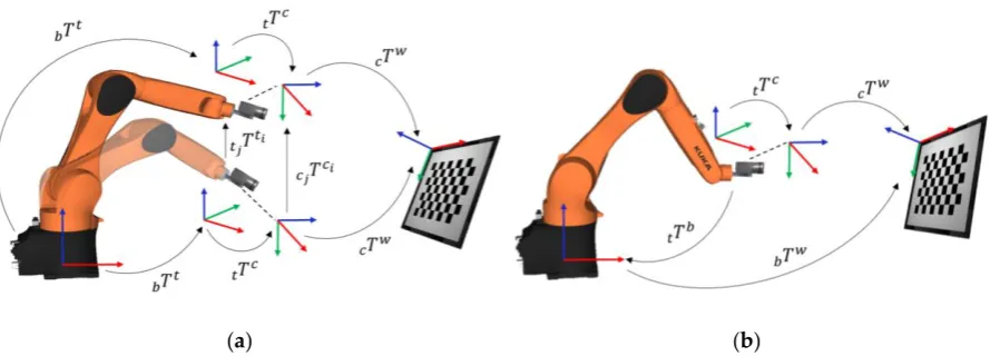
For the needs of our study, we introduce notations, as illustrated in Figure 1. Throughout this article, we will represent homogenous transformations by 𝑻 supported with various sub-indexes. The sub-indexes b, t, c and w indicate the coordinate frames associated with robot base, robot tool, camera and the calibration pattern, respectively. The sub-indexes i and j are associated with time instants of the state of the system. For the first general formulation 𝑨𝑿 = 𝑿𝑩 illustrated in Figure 1.a, 𝑻𝒕𝒊
𝒃 is the equivalent to 𝑨𝒊 and denotes the homogenous transformations from robot base to
the tool center point (TCP)/end-effector. 𝑻𝒘
𝒄𝒊 is the equivalent of 𝑩𝒊 and denotes the homogenous
transformation from camera to the world/calibration pattern. The formulation uses the relative transformation 𝑨 ( 𝑻𝒕𝒊)
𝒕𝒋 and 𝑩 ( 𝑻𝒄𝒋 𝒄𝒊) from their respective previous pose to another pose. The
unknown 𝑿 or 𝑻𝒄
The second general formulation, 𝑨𝑿 = 𝒁𝑩 is illustrated in Figure 1.b. The formulation uses absolute transformation 𝑨( 𝑻𝒃)
𝒕 and 𝑩( 𝑻𝒄 𝒘) from their respective coordinate frames. The
unknown 𝑿( 𝑻𝒘)
𝒃 and 𝒁( 𝑻𝒕 𝒄) are the homogenous transformations from robot base to the world
frame and the end effector to the camera frame, respectively. The hand-eye transformation is referred by Z in this formulation for coherence in literature, since many studies opt for such notation.
(a) (b)
Figure 1. Formulations relating geometrical transformation for calibration (a) Hand-eye calibration (b)
Robot-world-hand-eye Calibration
In this section, we focus on various cost functions for the two general problem formulations with the aim to analyze their performance under real situations. For both cases, we consider solving the problem by minimizing pose error and reprojection error. Some studies including [19] propose to
optimize the camera’s intrinsic parameters using the nonlinear solver to yield better results. However, Koide and Menegatti [21] argue that the approach involving camera intrinsic optimization overfits the model on the data for the reprojection error; consequently, the results are poor for other error metrics including reconstruction accuracy. Following the insight from [21], we solve for the transformation by minimizing the reprojection error.
2.1. Hand-Eye Formulation
This mathematical problem formulation involves estimating one unknown with the help of two known homogenous transformations in a single equation. Let 𝑻𝒕𝒊
𝒃 be the homogenous
transformation from the base of the robot to the robot TCP. The homogenous transformation relating the camera coordinate frame to the world coordinate frame affixed to the calibration patters is 𝑻𝒘
𝒄𝒊 .
The unknown homogenous transformation from the tool to the camera coordinate frame to be estimated is represented by 𝑻𝒄
𝒕 . Then from Figure 1.a, we can form the following relationship
𝑻𝒕𝟐 𝒃 −𝟏 𝑻𝒕𝟏 𝒃 𝑻𝒕 𝒄= 𝑻𝒕 𝒄 𝑻𝒄𝟐 𝒘 𝑻 𝒘 𝒄𝟏 −𝟏 ← ( 𝑻𝒄𝟏 𝒕𝟏 = 𝑻 𝒄𝟐
𝒕𝟐 ) (1) 𝑻𝒃 𝒕𝟐 𝑻 𝒕𝟏 𝒃 𝑻𝒕 𝒄= 𝑻𝒕 𝒄 𝑻𝒄𝟐 𝒘 𝑻 𝒄𝟏 𝒘 (2)
Generalizing Equation (2) gives us Equation (3).
𝑻𝒕𝒊
𝒕𝒋 𝑻
𝒄
𝒕 = 𝑻𝒕 𝒄 𝑻𝒄𝒋 𝒄𝒊 (3)
[ 𝑹
𝒕𝒊
𝒕𝒋 𝒕
𝒕𝒊
𝒕𝒋 01×3 1
] [ 𝒕𝑹𝒄 𝒕𝒕𝒄
01×3 1
] =[ 𝒕𝑹𝒄 𝒕𝒕𝒄
01×3 1
] [ 𝑹
𝒄𝒊
𝒄𝒋 𝒕
𝒄𝒊
𝒄𝒋 01×3 1
] (4)
Equation (4) represents the direct geometrical relationship between various coordinate frames involved in the system. In order to attain a solution and achieve dependable results it is required that the data is recorded for at least 3 positions with non-parallel movements of the rotational axis [14]. We can directly minimize the relationship in Equation (4) to estimate the unknown parameters presented in Equation (5). In the experimentation section, we refer to the cost functions in Equation (5) and (6) to as Xc1 and Xc2, respectively.
{𝑞(𝑡,𝑐), 𝒕𝒕 𝒄} =argmin 𝑞(𝑡,𝑐) , 𝑡𝑡𝑐
∑ ‖𝑛̅( 𝑻𝒕𝒊
𝒕𝒋 [𝑞(𝑡,𝑐), 𝒕
𝒄
𝒕 ]𝐻𝑇− [𝑞(𝑡,𝑐), 𝒕𝒕 𝒄]𝐻𝑇 𝒄𝒋𝑻𝒄𝒊 )‖2
2 𝑛−1
𝑖=1,𝑗=𝑖+1 (5)
In light of recommendation of [19], we can also re-arrange Equation (5) in the following manner.
{𝑞(𝑡,𝑐), 𝒕𝒕 𝒄} =argmin 𝑞(𝑡,𝑐) , 𝑡𝑡𝑐 ∑ ‖𝑛̅( 𝑻𝒕𝒊 𝒕𝒋 − [𝑞(𝑡,𝑐), 𝒕 𝒄 𝒕 ]𝐻𝑇 𝒄𝒋𝑻𝒄𝒊 [𝑞̃(𝑡,𝑐), 𝒕̃ 𝒄 𝒕 ]𝐻𝑇)‖ 2 2 𝑛−1
𝑖=1,𝑗=𝑖+1 (6)
Here, the symbol [ ]𝐻𝑇 denotes the conversion of the parameters to homogenous transformation representation. The solver optimizes the parameters in quaternion representation𝑞(𝑡,𝑐)
of the rotational matrix 𝑹𝒄
𝒕 and translation 𝒕𝒕𝒄. The operation 𝑛̅ denotes the aggregation of the
4x4-error matrix into a scalar value by summation of normalized values of quaternion angles and normalized translation vector. The terms 𝑞̃(𝑡,𝑐) and 𝒕𝒕̃𝒄 are the quaternion and translation vector
obtained from the inverse of 𝑻𝒄
𝒕 . The objective functions minimize the L2-norm of the residual
scaler values. The solutions in Equation (5) and (6) belong to the simultaneous solution category of hand-eye calibration because the rotation and translation are solved at the same time. We use the Levenberg –Marquardt algorithm to search for a minimum in the search space. The objective function successfully converges to a solution without any initial estimates for the 𝑞(𝑡,𝑐) and 𝒕𝒕𝒄. We have
observed that the cost function in Equation (6) enjoys a slight improvement in some cases over Equation (5), which will be discussed in the experimental results and discussion section.
The second approach to seek a solution is based on reprojection-based methods. Reprojection error minimization has shown promising results for pose estimation in various problem cases [25, 26]. Tabb [19] examined the reprojection-based method for the 𝑨𝑿 = 𝒁𝑩 formulation. We generalize this approach for the case of the 𝑨𝑿 = 𝑿𝑩 formulation. Let W be the 3D points in the world frame and 𝑃𝑐be the same points in the camera frame. In the case of the chessboard pattern, these points are
{𝑞(𝑡,𝑐), 𝒕𝒕𝒄} =argmin 𝑞(𝑡,𝑐) , 𝑡𝑡𝑐 ∑ ‖ 𝑃̅𝑗 − Π( 𝐾, [𝑞̃(𝑡,𝑐), 𝒕̃𝒕𝒄]𝐻𝑇 𝑻 𝒕𝒋 𝒕𝒊 [𝑞(𝑡,𝑐), 𝒕 𝒄 𝒕 ]𝐻𝑇 , 𝑃𝒊𝒄) ‖ 2 2 𝑛−1
𝑖=1,𝑗=𝑖+1 . (7)
In the equation, Π represents the operation that projects the 3D points from world space to image space using the camera intrinsic K and the camera extrinsic obtained using the homogenous transformations given in Equation (7), while 𝑃̅𝑗 are the observed 2D points in the j-th image.
It is important to note that the reprojection error minimization based approach is not invariant to the choice of initial estimates for the solver. However, if a good initial estimate is provided, the nonlinear optimization of reprojection error can provide a more accurate solution with a fine resolution.
2.2. Robot-World-Hand-Eye Formulation
This mathematical formulation involves the estimation of an additional homogenous transformation that is between the robot base frame and world frame. Therefore, we have two known and two unknown homogenous transformations. Let 𝑻𝒃
𝒕 be the homogenous transformation from
robot TCP to the base of the robot. The homogenous transformation relating the camera coordinate frame to the world coordinate is 𝑻𝒘
𝒄 .The additional unknown homogenous transformation from the
robot base frame to the world frame is 𝑻𝒘
𝒃 . Then from Figure 1.b, we can form a straightforward
geometrical relationship as:
𝑻𝒃
𝒕 𝒃𝑻𝒘= 𝑻𝒕 𝒄 𝑻𝒄 𝒘 (8)
[𝒕𝑹𝒃 𝒕𝒕𝒃
01×3 1
] [𝒃𝑹𝒘 𝒃𝒕𝒘
01×3 1
] =[ 𝒕𝑹𝒄 𝒕𝒕𝒄
01×3 1
] [𝒄𝑹𝒘 𝒄𝒕𝒘
01×3 1
] . (9)
Similar to the previous cases, we can directly use the relationship in aforementioned equations to obtain 𝑻𝒄
𝒕 and𝒃𝑻𝒘 using nonlinear minimization of their respective costs
{𝑞(𝑡,𝑐), 𝒕𝒕 𝒄, 𝑞(𝑏,𝑤), 𝒕𝒃𝒘} = argmin 𝑞(𝑡,𝑐) , 𝑡𝑡𝑐, 𝑞(𝑏,𝑤), 𝑡𝑏𝑤
∑ ‖𝑛̅( 𝑻𝒕 𝒊𝒃 [𝑞(𝑏,𝑤), 𝒕𝒃𝒘]𝐻𝑇− [𝑞(𝑡,𝑐), 𝒕𝒕 𝒄]𝐻𝑇 𝒄𝑻𝒊𝒘 )‖ 2 2 𝑛
𝑖=1 . (10)
We can observe from Equation (10), that we are attempting to solve for two unknown homogenous transformations. The adopted parametrization involves optimizing over 14 parameters, where the two quaternions and translation vectors contribute to 8 and 6 parameters, respectively. Although the robot-world-hand-eye calibration involves more unknowns for estimation, nonetheless, it constrains the geometry with more anchor points and helps to converge closer to the global minimum. With the advent of modern nonlinear solvers, the problem of optimizing for a large number of unknowns has become simpler and more efficient. As before, the objective function in Equation (10) can be re-arranged in the form of Equation (11). The cost functions in Equation (10) and (11) are referred to as Zc1and Zc2, respectively, in Tabb [19]
{𝑞(𝑡,𝑐), 𝒕𝒕 𝒄, 𝑞(𝑏,𝑤), 𝒕𝒃 𝒘} = argmin 𝑞(𝑡,𝑐) , 𝑡𝑡𝑐, 𝑞(𝑏,𝑤), 𝑡𝑏𝑤 ∑ ‖𝑛̅( 𝑻𝒊𝒃 𝒕 − [𝑞(𝑡,𝑐), 𝒕𝒕 𝒄]𝐻𝑇 𝑻 𝒄 𝒘𝒊 [𝑞̃(𝑏,𝑤), 𝒕̃𝒃 𝒘]𝑯𝑻)‖ 2 2 𝑛
𝑖=1 . (11)
The objective function successfully converges to a solution for 𝑞(𝑡,𝑐), 𝒕𝒕 𝒄, 𝑞(𝑏,𝑤) and 𝒃𝒕𝒘.
However, the primary difference here is that the solver depends on good initialization. In case of bad initial estimates, the optimization algorithm might not converge to a stable solution.
This formulation can also be viewed as reprojection error minimization problem. The following equation presents a cost function that minimizes the reprojection of the 3D world points 𝑊 onto the image space in camera frame, where 𝑃̅𝑖 are the observed 2D points in the i-th image. The cost
functions in Equation (12) is referred to as rp1 in [19].
{𝑞(𝑡,𝑐), 𝒕𝒕 𝒄, 𝑞(𝑏,𝑤), 𝒕𝒃 𝒘} = argmin 𝑞(𝑡,𝑐) , 𝑡𝑡𝑐, 𝑞(𝑏,𝑤), 𝑡𝑏𝑤
∑ ‖ 𝑃̅𝑖− Π( 𝐾, [𝑞̃(𝑡,𝑐), 𝒕̃𝒕 𝒄]𝐻𝑇 𝑻𝒕 𝒊𝒃 [𝑞(𝑏,𝑤), 𝒕𝒃𝒘]𝐻𝑇, 𝑊) ‖2 2 𝑛
In contrast to the reprojection error cost function for problem formulation = 𝑋𝐵 , this formulation from [19] has the added advantage that it is not explicitly affected by the errors in pose estimation caused by blurred images or low camera resolution. If the camera intrinsic parameters are accurate enough, then the extrinsic can be indirectly computed as a transformation through 𝑻𝒄
𝒕 , 𝑻𝒕 𝒃
and 𝑻𝒘
𝒃 through the minimization of the objective function. On the contrary, the reprojection error
cost function presented for problem formulation 𝑨𝑿 = 𝑿𝑩 is more robust to robot pose errors given good images.
A marginal improvement in the results can be observed in various cases by using log(cosh(𝑥))
as the loss function. The relative improvement is discussed in detail in Section 5. log(cosh(𝑥))
approximates 𝑥22 for small value of 𝑥 and 𝑎𝑏𝑠(𝑥) − log(2), for large values. This essentially means that log(cosh(𝑥)) imitates the behavior of the mean squared error but is more robust to noise and outliers. Moreover, the function is twice differentiable everywhere and therefore does not deteriorate the convexity of the problem. The modified version is given as followed, where 𝐸(𝑥) is the error in terms of difference between the observed points and the reprojected points. The cost function in Equation (13) is referred to as RZ hereafter.
{𝑞(𝑡,𝑐), 𝒕𝒕 𝒄, 𝑞(𝑏,𝑤), 𝒕𝒃 𝒘} = argmin 𝑞(𝑡,𝑐) , 𝑡𝑡𝑐, 𝑞(𝑏,𝑤), 𝑡𝑏𝑤
∑𝑛𝑖=1‖ log(cosh( 𝐸(𝑥))) ‖22 (13)
3. Performance Evaluation using Datasets
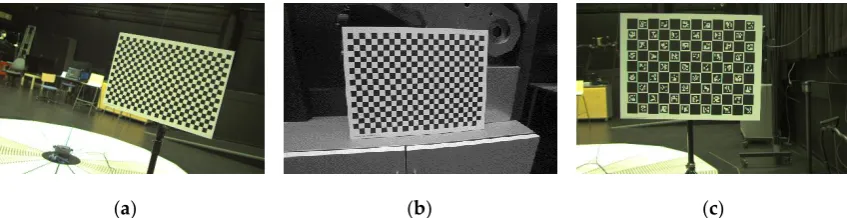
In order to assess the performance of the robot-world/hand-eye calibration methods, we present multiple datasets to test the methods in laboratory and near field settings. These datasets contain data acquired using various combinations of camera, lens, calibration patterns and robot poses. A detailed description of datasets is provide in Table 1. The table also lists the length of each side of square of the calibration patterns, focal length of the lenses, and number of robot poses used to acquire images. The datasets include real data and simulated data with synthetic images. To the best of our knowledge, this study is the first to provide simulated robot-world/hand-eye calibration dataset with synthetic/rendered images as open source for public use. A more detailed explanation of the datasets is presented in the following subsections.
Table 1. Description of the dataset acquired and generated for testing.
No. Dataset Data Type Lens focal length [mm]
Square
Size [mm] Image Size Robot Poses
1 kuka_1 Real 12 20 1928 x 1208 KR16L6-2 30
2 kuka_2 Real 16 15 1920 x 1200 KR16L6-2 28
3 kuka_3 Real 12 60 1928 x 1208 KR16L6-2 29
4 CS_synthetic_1 Simulated 18 200 1920 x 1080 N/A 15
5 CS_synthetic_2 Simulated 18 200 1920 x 1080 N/A 19
6 CS_synthetic_3 Simulated 18 200 1920 x 1080 N/A 30
3.1 Real Datasets
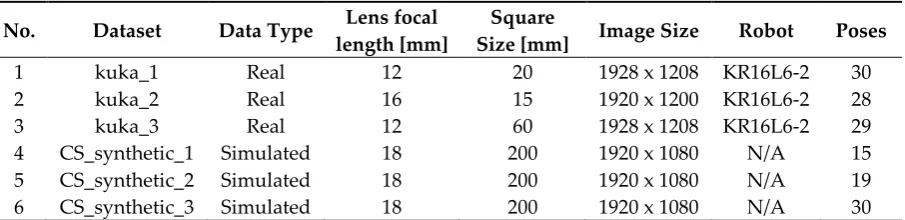
To acquire real data for this experiment, a KUKA KR16L6-2 serial 6-DOF robot arm was used with Basler acA1920-50gc camera using 12 mm and 16 mm lenses as shown in Figure 2. The primary aim in recording these datasets was to collect real data for various robot-world/hand-eye calibration tests. With this aim, the collection provides three real datasets with varying robot poses and calibration patterns as shown in Figure 3. In this study, we primarily use the chessboard pattern for accurate camera calibration and robot-world/hand-eye calibration. A minor yet significant difference between the datasets [27], used in [19], is that the robot hand/camera orientation changes are quite gentle. This is done to facilitate the OpenCV camera calibration implementation used in [19], therefore the aforementioned implementation is not invariant to significant orientation changes and as a result, it flips the origin of the calibration pattern. For our experiments, we utilized MATLAB’s
However, this neat trick requires that the calibration pattern is asymmetric in the number of rows and columns and that one of the sides has an even number of squares while the other side has odd. This requirement makes the datasets in [27], which have chessboard patterns with even number of rows and columns, unusable in our tests.
In addition, the calibration board used in the third dataset is a ChArUco pattern with square size of 60mm, shown in Figure 3.c. ChArUco tries to combine the benefit of both chessboard and ArUco markers and tends to facilitate the calibration process by fast, robust and accurate corner detection even in occluded or partial views [28]. The ChArUco dataset is only provided as open source material for future testing and has not been utilized in this study.
(a) (b)
Figure 2. An example of the setup for acquiring the datasets (a) Robotic arm moving in the workspace (b)
Cameras and Lenses for data acquisition
(a) (b) (c)
Figure 3. Example of captured images from the dataset 1 through 3.
3.2 Simulated Dataset with Synthetic Images
(a) (b) (c)
Figure 4. Example of rendered images for simulated dataset from the dataset 4 through 6.
3.3 Pseudo-Real Noise Modeling
Although simulated data carries the advantage of providing the ground truth information for various robot-world/hand-eye calibration, the limitation is that it lacks the uncertainties of the real world situations. These uncertainties could originate from either robot TCP pose errors or camera pose errors. Many studies [19, 21, 30] suggest testing the robustness of the methods by inducing one type of noise at a time into the system and evaluating its performance based on the response. Unfortunately, these uncertainties are mostly co-existent and co-dependent in real-world cases. In this study, we propose to model the uncertainties in terms of pose and pixel errors and induce a realistic amount of noise simultaneously into the simulated dataset for testing. The motivation behind inducing such type of noise is to carry the advantage of testing simulated data for accuracy and adjoining it with the robustness of testing on real data.
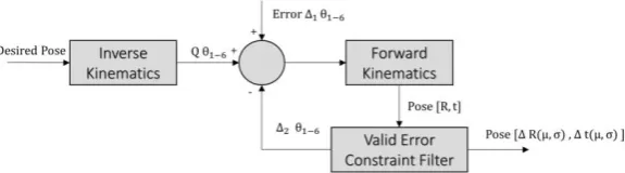
We aim at introducing a realistic amount of noise. The robot position repeatability is generally provided in the datasheets, which ranges from 0.1mm-0.3mm for various robots. However, the orientation repeatability is absent since it cannot be measured for real robots at such a fine resolution. Here, we propose a reverse engineering approach to acquire a statistically valid amount of orientation noise. The position and orientation error of the TCP arises from the accumulated errors of the individual joints of the robotic arm due to robot flexibility and backlash. Using inverse kinematic we can find the joint angles for any position of TCP within its workspace.
Once the joint angles are available, we can introduce noise into the individual joints through trial and error until it produces the end-effector position error comparable to the realistic error. Through forward kinematics, we can then estimate the position and orientation of the end-effector under various arm configurations. Figure 5 shows the operation flow for computing the error range of the new orientations.
Figure 5. Flowchart of the orientation noise modelling approach
(a) (b)
Figure 6. Probability Distributions Functions (a) The measured position error from the robotic arm (b) The
modeled orientation error for the robotic arm.
4. Error Metrics
In order to compare the results of all the methods with other existing studies, we suggest to use mean rotation error (deg), mean translation error (mm), reprojection error (px), absolute rotation error (deg), and absolute translation error (mm). Each error metric has its own merits and demerits. We have avoided the use of reconstruction error since it involves further estimation of valid 3D points from the reprojected 2D points. This can be achieved by searching the space for such 3D points using nonlinear minimization, as before. However, it is not possible to segregate the error that arises from the pose estimation step and the reconstruction step, while using the error metric.
The first error is the mean rotation error derived from Equation (4) and (9) for 𝑨𝑿 = 𝑿𝑩 and
𝑨𝑿 = 𝒁𝑩 formulation, respectively. Equation (16) gives the mean rotation error, which takes its input from Equation (14) and (15) for their respective formulation. Here, the angle represents the conversion from a rotation matrix to axis-angle for simpler user interpretation.
∆𝑹 = ( 𝑹𝒄 𝒕 𝑹𝒄 𝒘 )
−1
𝑹𝒃
𝒕 𝒃𝑹𝒘 (14)
∆𝑹 = ( 𝑹𝒄 𝒕 𝑹𝒄𝒋 𝒄𝒊 )
−1
𝑹𝒕𝒊
𝒕𝒋 𝑹
𝒄
𝒕 (15)
𝑒𝑟𝑅=1𝑛∑𝑛𝑖=1‖𝑎𝑛𝑔𝑙𝑒(∆𝑹)‖22 (16)
The second error metric focuses on computing the translation errors. As above, the translation errors
emerge from the same Equation (4) and (9).
𝑒𝑟𝑡=1𝑛∑ ‖( 𝑹𝒕𝒋 𝒕𝒊 𝒕
𝒄)
𝒕 + 𝒕𝒕𝒋 𝒕𝒊− ( 𝑹
𝒄 𝒕𝒄𝒊)
𝒄𝒋
𝒕 + 𝒕𝒕 𝒄‖ 2 2 𝑛−1
𝑖=1,𝑗=𝑖+1 (17)
𝑒𝑟𝑡=1𝑛∑ ‖( 𝑹𝒕 𝒃 𝒕𝒃𝒘)+ 𝒕𝒕 𝒃− ( 𝑹𝒕 𝒄 𝒕𝒄 𝒘)+ 𝒕𝒕 𝒄‖2 2 𝑛
𝑖=1 (18)
The third metric to measure the quality of the results is the reprojection root mean squared error (𝑟𝑟𝑚𝑠𝑒).The 𝑟𝑟𝑚𝑠𝑒 is measured in pixels and is a good metric to measure the quality of the results in the absence of ground truth information. The 𝑟𝑟𝑚𝑠𝑒 provides an added advantage that it back-projects the 3D points from the calibration board onto the images by first transforming them through the robotic arm. In case, if the hand eye calibration is not correct, the reprojection errors will be large. The 𝑟𝑟𝑚𝑠𝑒 for both the formulations are given in Equation (19) and (20).
𝑒𝑟𝑟𝑚𝑠𝑒= √ 1
𝑛−1∑ ‖ 𝑃̅𝑗 − Π ( 𝐾, [𝑞̃(𝑡,𝑐), 𝒕̃ 𝒄
𝒕 ]𝐻𝑇 𝑻 𝒕𝒋 𝒕𝒊 [𝑞(𝑡,𝑐), 𝒕
𝒄
𝒕 ]𝐻𝑇 , 𝑃𝒊𝒄)‖2 2 𝑛−1
𝑖=1,𝑗=𝑖+1 (19)
𝑒𝑟𝑟𝑚𝑠𝑒= √1𝑛∑ ‖ 𝑃̅𝑖 − Π( 𝐾, [𝑞̃(𝑡,𝑐), 𝒕̃𝒕𝒄]𝐻𝑇 𝑻𝒕 𝒊𝒃 [𝑞(𝑏,𝑤), 𝒕𝒃𝒘]𝐻𝑇 , 𝑊) ‖2 2 𝑛
For the case of simulated data, we have accurate ground truth pose from the robot TCP to the camera. We can effectively utilize that information to acquire the absolute rotation error and absolute translation errors. The absolute rotation error can be obtained using Equation (21), while the absolute translation error is given using Equation (22). Here, 𝒕𝑹𝒈𝒕𝒄 and 𝒕𝒕𝒈𝒕𝒄 are the ground truth values.
𝑒𝑎𝑅= ‖𝑎𝑛𝑔𝑙𝑒( 𝑹𝒕 𝒄−1 𝑹𝒕 𝒈𝒕𝒄 )‖2 2
(21)
𝑒𝑎𝑡= ‖ 𝒕𝒕 𝒈𝒕𝒄 − 𝒕𝒕 𝒄)‖2 2
(22)
5. Experimental Results and Discussion
In this section, we report the experimental results for various cases and discuss the obtained results. We tabulate the results obtained for these cases using our own and six other studies to provide a clear comparison. Table 1 through 4 summarizes the results using the error metrics described in Section 4, over the datasets presented in Section 3. To elaborate on the naming, Xc1, Xc2, RX, and RZ refer to the optimization of the cost function based on Equation (5-7) and (13), respectively. In addition, Figure 7 illustrates the results from simulated data in dataset 5 over varying visual noise. The curves represent the averaged results over 1000 iterations in order to achieve a stable response. It is noteworthy, that the visual noise is varied in the presence of the pseudo-realistic robotic arm pose noise.
Table 2 and 3 shows the evaluation of the aforementioned methods on dataset 1 and 2, respectively. Both datasets vary in the use of camera lenses and robot arm poses. However, the number of poses and camera resolution remain almost same. It can be observed that the method by Shah [8] provides a better distribution of the rotational error and hence has the lowest relative rotation error (𝑒𝑟𝑅) values, while the method by Li et al. [9] yields a comparable result. The lowest
relative translation error (𝑒𝑟𝑡) varies for both datasets and is yielded by the proposed method Xc2
and Park and Martin [31]. However, for dataset 2, it seems that Xc2 has not converged properly and has obtained a local minimum. On the other hand, the method by Park and Martin [31], still yields a relatively low 𝑒𝑟𝑡. Moreover, for both datasets 1 and 2, the method by Horaud and Dornaika [11]
provides comparable results to Park and Martin [31].
For the reprojection root mean squared error 𝑒𝑟𝑟𝑚𝑠𝑒, the best results are obtained using the
proposed RX approach for both tests. This is aided by the fact that the recorded datasets do not have large visual errors and as a result, RX performs comparably better. Moreover, since the cost function has only one unknown transformation to minimize for, the optimizer distributes the errors more evenly for the reprojection based cost function. Other reprojection based approaches namely Tabb’s
rp1 [19] and RZ achieve quite close results to RX. It is noteworthy, that in spite of being a closed-form approach, Shah [8] obtains quite good 𝑒𝑟𝑟𝑚𝑠𝑒 that are at a competitive level to the reprojection errors
Table 2 Comparison of methods using the described error metrics for Dataset 1.
Method Evaluation
Form
Relative Rotation (𝒆𝒓𝑹)
Relative Translation (𝒆𝒓𝒕)
Reprojection Error 𝒆𝒓𝒓𝒎𝒔𝒆
Tsai [3] AXXB 0.051508 1.1855 2.5386
Horaud and
Dornaika [11] AXXB 0.051082 1.0673 2.5102
Park and Martin [31] AXXB 0.051046 1.0669 2.5091
Li et al. [9] AXZB 0.043268 1.6106 2.5135
Shah [8] AXZB 0.042594 1.5907 2.4828
Xc1 AXXB 0.11619 7.0582 17.806
Xc2 AXXB 0.075211 0.71369 3.3834
Tabb Zc1 [19] AXXB 0.051092 1.1315 2.5796
Tabb Zc2 [19] AXZB 0.10205 3.6313 5.2324
RX AXXB 0.076491 1.7654 2.3673
Tabb rp1 [19] AXZB 0.066738 1.9455 2.4004
RZ AXZB 0.079488 2.0806 2.4114
Table 3 Comparison of methods using the described error metrics for Dataset 2.
Method Evaluation
Form
Relative Rotation (𝒆𝒓𝑹)
Relative Translation (𝒆𝒓𝒕)
Reprojection Error 𝒆𝒓𝒓𝒎𝒔𝒆
Tsai [3] AXXB 0.046162 0.48363 1.9944
Horaud and
Dornaika [11] AXXB 0.042587 0.4104 1.3804
Park and Martin [31] AXXB 0.042639 0.41033 1.3807
Li et al. [9] AXZB 0.040297 39.535 61.466
Shah [8] AXZB 0.04028 0.6078 1.5767
Xc1 AXXB 1.2697 10.038 54.436
Xc2 AXXB 9.7461 24.908 197.96
Tabb Zc1 [19] AXXB 0.61435 4.9182 16.103
Tabb Zc2 [19] AXZB 0.48439 13.518 23.672
RX AXXB 0.092173 0.6726 1.1234
Tabb rp1 [19] AXZB 0.16515 0.84439 1.1438
RZ AXZB 0.14824 0.81163 1.1567
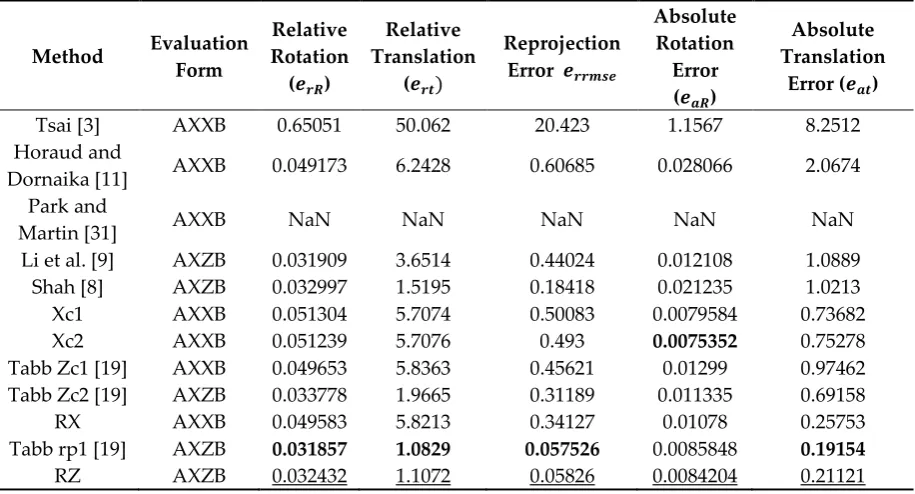
In addition to the previous tabulated results, Table 4 and 5 provide experimental results on simulated data with synthetic images. Table 4 and 5 both provide test results on dataset 6. The main difference between the two tests is that the first test (Table 4) considers ideal simulated data, while the second test (Table 5) has visual and robot pose noise induced. The robot pose noise is derived from the process explained in Section 3.3, while the visual noise is selected such that the resultant reprojection error amounts to the reprojection errors of real data tests.
Table 4 and 5, present two absolute errors due to the presence of ground truth information for the simulated cases. It can be observed that Tabb’s rp1 [19] achieves the least 𝑒𝑟𝑅, 𝑒𝑟𝑡, 𝑒𝑟𝑟𝑚𝑠𝑒 and 𝑒𝑎𝑡.
Xc2 yields minimum Absolute Rotation Error (𝑒𝑎𝑅). For this dataset, the method by Park and Martin
[31], failed to find a solution as it suffered from singularity. It is important to note for an ensued comparison that the proposed method RZ yields the second best results over most of the error metrics with minor differences from the least errors. This is important in a sense that all the errors are equally distributed and restricted close to their minimum values.
The backend experiments for the results in Table 5 use the same methods, metrics and dataset, as for Table 4. In agreement with the results of real data, Shah [8]yields the least 𝑒𝑟𝑅 for this dataset
proposed method RZ yields the minimum 𝑒𝑟𝑡, 𝑒𝑟𝑟𝑚𝑠𝑒 and, 𝑒𝑎𝑡 and the second best result for𝑒𝑎𝑅.
Tabb Zc1 [19] obtains the minimum 𝑒𝑎𝑅.
This comparison demonstrates that the proposed RZ is more robust to outliers present in the data and performs marginally better compared to Tabb’s rp1 [19] in the presence of noise.
Table 4 Comparison of methods using the described error metrics for Dataset 6.
Method Evaluation Form
Relative Rotation (𝒆𝒓𝑹)
Relative Translation
(𝒆𝒓𝒕)
Reprojection Error 𝒆𝒓𝒓𝒎𝒔𝒆
Absolute Rotation
Error (𝒆𝒂𝑹)
Absolute Translation
Error (𝒆𝒂𝒕)
Tsai [3] AXXB 0.65051 50.062 20.423 1.1567 8.2512
Horaud and
Dornaika [11] AXXB 0.049173 6.2428 0.60685 0.028066 2.0674
Park and
Martin [31] AXXB NaN NaN NaN NaN NaN
Li et al. [9] AXZB 0.031909 3.6514 0.44024 0.012108 1.0889
Shah [8] AXZB 0.032997 1.5195 0.18418 0.021235 1.0213
Xc1 AXXB 0.051304 5.7074 0.50083 0.0079584 0.73682
Xc2 AXXB 0.051239 5.7076 0.493 0.0075352 0.75278
Tabb Zc1 [19] AXXB 0.049653 5.8363 0.45621 0.01299 0.97462
Tabb Zc2 [19] AXZB 0.033778 1.9665 0.31189 0.011335 0.69158
RX AXXB 0.049583 5.8213 0.34127 0.01078 0.25753
Tabb rp1 [19] AXZB 0.031857 1.0829 0.057526 0.0085848 0.19154
RZ AXZB 0.032432 1.1072 0.05826 0.0084204 0.21121
Table 5 Comparison of methods using the described error metrics for Dataset 6 with robot pose and visual noise.
Method Evaluation Form
Relative Rotation (𝒆𝒓𝑹)
Relative Translation
(𝒆𝒓𝒕)
Reprojection Error 𝒆𝒓𝒓𝒎𝒔𝒆
Absolute Rotation Error (𝒆𝒂𝑹)
Absolute Translation
Error (𝒆𝒂𝒕)
Tsai [3] AXXB 34.925 2476.4 99190 28.04 747.48
Horaud and
Dornaika [11] AXXB 1.723 199.92 18.764 0.43124 47.913
Park and
Martin [31] AXXB 1.7208 199.98 18.916 0.43819 47.733
Li et al. [9] AXZB 1.177 80.061 7.8757 0.0029485 23.272
Shah [8] AXZB 1.1767 58.552 8.5123 0.51765 8.3389
Xc1 AXXB 1.7752 192.86 17.442 0.12827 37.068
Xc2 AXXB 1.8026 193.22 19.031 0.20831 40.4
Tabb Zc1 [19] AXXB 1.7989 206.01 13.445 0.0042828 11.368
Tabb Zc2 [19] AXZB 1.2571 86.844 13.891 0.050182 27.247
RX AXXB 1.8087 204.06 12.534 0.027714 7.0139
Tabb rp1 [19] AXZB 1.2093 44.982 1.5463 0.0075401 0.95904
RZ AXZB 1.2079 44.932 1.546 0.0069577 0.95845
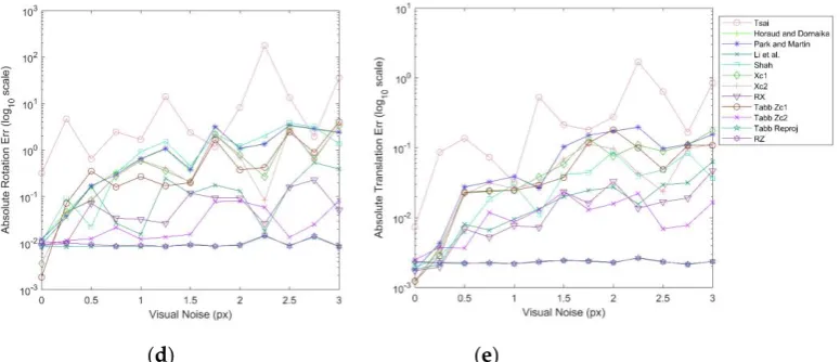
some magnitude of visual noise due to various reasons. The presence of visual noise may effect each method differently depending on the approach used. Nonetheless, the nonlinear reprojection based methods of the formulation 𝑨𝑿 = 𝒁𝑩 show good estimation results under visual noise and hand pose noise.
6. Conclusions
This study has examined the robot-world/hand-eye calibration problem in its two alternative geometrical interpretations, and has proposed a collection of novel methods It benefits from non-linear optimizers that iteratively minimize the cost function and determine the transformations. We have conducted a comparative study to quantify the performances of optimizing over pose errors and reprojection errors. The code for the presented methods is provided as open-source for further use. Our collection of methods was evaluated with respect to state-of-the-art methods. The study also contributes new datasets for testing and validation purposes. These include subsets of three real data and three simulated data with synthetic images. Simulated data are beneficial as they provide ground truth. We have proposed a noise modeling approach to generate realistic robot TCP orientation noise to study the robustness of methods under realistic conditions. We showed that our methods perform well under different testing conditions. RX yields good results with high accuracy under realistic visual noise with respect to reprojection error. In addition, RZ is more robust to visual noise and yields more consistent results for a greater range of visual noise.
(a) (b)
(d) (e)
Figure 7 Metric error results for Dataset 5 with constant robot pose noise (a) mean rotation error (b) mean
translation error (c) reprojection error (d) absolute rotation error against ground truth (e) absolute translation
error against ground truth.
Supplementary Materials: The dataset and the code is available from [32] for public use.
Funding: The work presented in this paper was funded by Fusion for Energy (F4E) and Tampere University under the F4E grant contract F4E-GRT-0901. The results are intended to be integrated in advanced camera-based systems attached to manipulator arms in order to achieve complex Remote Handling maintenance operations in a safe and efficient way.
Disclaimer: This article reflect the views of the authors. F4E and TUNI cannot be held responsible for any use which may be made of the information contained herein.
Conflicts of Interest: The authors declare no conflict of interest.
References
1. Levine, S.; Pastor, P.; Krizhevsky, A.; Ibarz, J.; Quillen, D. Learning hand-eye coordination for robotic grasping with deep learning and large-scale data collection. The International Journal of Robotics Research 2017, 37, 421-436, doi: 10.1177/0278364917710318.
2. Pachtrachai, K.; Allan, M.; Pawar, V.; Hailes, S.; Stoyanov, D. Hand-eye calibration for robotic assisted minimally invasive surgery without a calibration object. In International Conference on Intelligent Robots and Systems (IROS), Daejeon, South Korea,9-14 October 2016; pp. 2485-2491.
3. Tsai, R.; Lenz, R. A new technique for fully autonomous and efficient 3D robotics hand/eye calibration. IEEE Transactions on Robotics and Automation 1989, 5, 345-358, doi: 10.1109/70.34770.
4. Shiu, Y.; Ahmad, S. Calibration of wrist-mounted robotic sensors by solving homogeneous transform equations of the form AX=XB. IEEE Transactions on Robotics and Automation 1989, 5, 16-29, doi: 10.1109/70.88014.
5. Zhuang, H.; Roth, Z.; Sudhakar, R. Simultaneous robot/world and tool/flange calibration by solving homogeneous transformation equations of the form AX=YB. IEEE Transactions on Robotics and Automation 1994, 10, 549-554, doi: 10.1109/70.313105.
6. Liang, R.; Mao, J. Hand-eye calibration with a new linear decomposition algorithm. Journal of Zhejiang University-SCIENCE A 2008, 9, 1363-1368, doi: 10.1631/jzus.A0820318.
7. Hirsh, R.; DeSouza, G.; Kak, A. An iterative approach to the hand-eye and base-world calibration problem. In IEEE International Conference on Robotics and Automation, Seoul, South Korea, 21-26 May 2001;pp. 2171-2176.
8. Shah, M. Solving the Robot-World/Hand-Eye Calibration Problem Using the Kronecker Product. Journal of Mechanisms and Robotics 2013, 5, 031007, doi: 10.1115/1.4024473.
10. Chen, H. A screw motion approach to uniqueness analysis of head-eye geometry. In IEEE Computer Society Conference on Computer Vision and Pattern Recognition,Maui, USA, 3-6 June 1991; pp. 145-151. 11. Horaud, R.; Dornaika, F. Hand-Eye Calibration. The International Journal of Robotics Research 1995, 14,
195-210., doi: 10.1177/027836499501400301.
12. Shi, F.; Wang, J.; Liu, Y. An approach to improve online hand-eye calibration. In Pattern Recognition and Image Analysis, Proceedings of the Iberian Conference on Pattern Recognition and Image Analysis, Estoril, Portugal, 7–9 June 2015; Springer: Berlin/Heidelberg, Germany, 2005; pp. 647–655.
13. Wei, G.; Arbter, K.; Hirzinger, G. Active self-calibration of robotic eyes and hand-eye relationships with model identification. IEEE Transactions on Robotics and Automation 1998, 14, 158-166, doi: 10.1109/70.660864. 14. Strobl, K.H.; Hirzinger, G. Optimal hand-eye calibration. In Proceedings of the 2006 IEEE/RSJ International
Conference on Intelligent Robots and Systems, Beijing, China, 9–15 October 2006; pp. 4647–4653.
15. Fassi, I.; Legnani, G. Hand to sensor calibration: A geometrical interpretation of the matrix equation. Journal of Robotic Systems 2005, 22, 497-506, doi: 10.1002/rob.20082.
16. Zhao, Z. Hand-eye calibration using convex optimization. In IEEE International Conference on Robotics and Automation, Shanghai, China, 9–13 May 2011; pp. 2947–2952.
17. Heller, J.; Havlena, M.; Pajdla, T. Globally Optimal Hand-Eye Calibration Using Branch-and-Bound. IEEE
Transactions on Pattern Analysis and Machine Intelligence 2016, 38,1027-1033, doi:
10.1109/TPAMI.2015.2469299.
18. Hartley, R.; Kahl, F. Global Optimization through Rotation Space Search. International Journal of Computer Vision 2009, 82, 64-79, doi: 10.1007/s11263-008-0186-9.
19. Tabb, A.; Ahmad Yousef, K. Solving the robot-world hand-eye(s) calibration problem with iterative methods. Machine Vision and Applications 2017, 28, 569-590, doi: 10.1007/s00138-017-0841-7.
20. Agarwal, S. and Mierle, K. Ceres Solver — A Large Scale Non-linear Optimization Library. [online] Ceres-solver.org. Available at: http://ceres-solver.org/.
21. Koide, K.; Menegatti, E. General Hand–Eye Calibration Based on Reprojection Error Minimization. IEEE Robotics and Automation Letters 2019, 4, 1021-1028, doi: 10.1109/lra.2019.2893612.
22. Zhi, X.; Schwertfeger, S. Simultaneous hand-eye calibration and reconstruction. In International Conference on Intelligent Robots and Systems (IROS) 2017,Vancouver, BC, Canada,24-28 September 2017; pp. 1470-1474.
23. Li, W.; Dong, M.; Lu, N.; Lou, X.; Sun, P. Simultaneous Robot–World and Hand–Eye Calibration without a Calibration Object. Sensors 2018, 18, 3949, doi: 10.3390/s18113949.
24. Zhang, Z. A flexible new technique for camera calibration. IEEE Transactions on Pattern Analysis and Machine Intelligence 2000, 22, 1330-1334, doi: 10.1109/34.888718.
25. Edlund, O. A software package for sparse orthogonal factorization and updating. ACM Transactions on Mathematical Software 2002, 28, 448-482, doi: 10.1145/592843.592848.
26. Hesch, J.; Roumeliotis, S. A Direct Least-Squares (DLS) method for PnP. In International Conference on Computer Vision 2011,Barcelona, Spain,6-13 November 2011; pp. 383-390.
27. Tabb, A. Data from: Solving the Robot-World Hand-Eye(s) Calibration Problem with Iterative Methods, National Agricultural Library http://dx.doi.org/10.15482/USDA.ADC/1340592 (accessed Apr 28, 2019). 28. OpenCV: Detection of ChArUco Corners https://docs.opencv.org/3.1.0/df/d4a/tutorial_charuco_detection (accessed Apr 28, 2019).
29. Foundation, B. blender.org - Home of the Blender project - Free and Open 3D Creation Software https://www.blender.org/ (accessed Apr 28, 2019).
30. Lee, J.; Jeong, M. Stereo Camera Head-Eye Calibration Based on Minimum Variance Approach Using Surface Normal Vectors. Sensors 2018, 18, 3706, doi: 10.3390/s18113706.
31. Park, F.; Martin, B. Robot sensor calibration: solving AX=XB on the Euclidean group. IEEE Transactions on
Robotics and Automation 1994, 10, 717-721, doi: 10.1109/70.326576.