wave generation in depth averaged, shallow water models, they have not seen the same level of adoption

The Efficient Application of an Impulse Source

Wavemaker to CFD Simulations

Pál Schmitt1* , Christian Windt2Josh Davidson2, John V. Ringwood2and Trevor Whittaker1

1 _{Marine Research Group, Queen’s University Belfast, BT9 5AG Belfast, Northern Ireland; p.schmitt@qub.ac.uk}

2 _{Centre for Ocean Energy Research, Maynooth University, Ireland; e-mail@e-mail.com}

* Correspondence: p.schmitt@qub.ac.uk;

Version January 22, 2019 submitted to Preprints

Abstract:Computational Fluid Dynamics (CFD) simulations, based on Reynolds Averaged Navier Stokes

1

(RANS) models, are a useful tool for a wide range of coastal and offshore applications, providing a high

2

fidelity representation of the underlying hydrodynamic processes. Generating input waves in the CFD

3

simulation is performed by a numerical wavemaker (NWM), with a variety of different NWM methods

4

existing for this task. While NWMs, based on impulse source methods, have been widely applied for

5

wave generation in depth averaged, shallow water models, they have not seen the same level of adoption

6

in the more general RANS based CFD simulations, due to difficulties in relating the required impulse

7

source function to the resulting free surface elevation for non-shallow water cases. This paper presents

8

an implementation of an impulse source wavemaker, which is able to self-calibrate the impulse source

9

function to produce a desired wave series in deep or shallow water at a specific point in time and space.

10

Example applications are presented, for a numerical wave tank (NWT), based on the opensource CFD

11

software OpenFOAM, for wave packets in deep and shallow water, highlighting the correct calibration of

12

phase and amplitude. Also, the suitability for cases requiring very low reflection from NWT boundaries is

13

demonstrated. Possible issues in the use of the method are discussed and guidance for good application

14

is given.

15

Keywords:numerical wave tank; internal wavemaker; CFD ; wave generation; OpenFOAM

16

1. Introduction 17

While CFD enables the simulation of complex flow phenomena, such as two-phase flows and gravity

18

waves, setting up a simulation of coastal or marine engineering processes, with correct wave creation and

19

minimum reflection, can be a challenge. A wide range of NWM methods exist in the literature for the

20

generation and absorption of waves in a CFD simulation.

21

Wave generation methods can be broadly grouped into two main categories:

22

1. Replication of physical wavemakers, such as oscillating flaps, paddles or pistons

23

2. Implementation of numerical/mathematical techniques, introducing source terms or similar into the

24

governing equations

25

The first category of wave generation methods directly simulates the wavemaker by a moving wall,

26

requiring mesh motion/deformation in the CFD domain [?], which can be a complex and computationally

27

expensive task. Additionally, because these methods replicate the real processes in a physical laboratory

28

tank, they also incur the well known drawbacks of physical wavemakers encountered in an experimental

29

facility, such as evanescent waves, imperfect wave absorption and the required implementation of a

30

wavemaker control system. Another drawback of conventional wave pistons is that they are typically

31

limited to low order waves (first or second order).

32

In contrast to directly mimicking physical wavemakers, the second category of wave generation

33

methods are generally more computationally efficient, using numerical algorithms to create the desired

34

flow conditions by manipulating the field variables. In principle there are four types of methods in the

35

second category of wave generators:

36

• relaxation method- relaxes the results of the simulation inside the domain with the results given by

37

wave theory [? ? ? ? ] (linear or higher order) or other numerical models like boundary element

38

methods (BEM) for example [? ?].

39

• boundary method- creates and absorbs waves on boundary patches through Dirichlet boundary

40

conditions [? ? ?]

41

• mass source method- the wave is created by adding a source term to the continuity equation [? ? ? ?]

42

• impulse source method- the wave is created by adding a source term to the impulse equation [? ? ? ?]

43

Correspondingly, wave absorption can also be achieved using a number of methods. The trivial

44

solution, of using a very long tank and limiting the simulation duration to a small number of wave

45

cycles, is certainly not efficient or elegant and will therefore not be considered herein. The relaxation and

46

boundary wave generation methods, allow for wave absorption to be achieved actively by the NWM,

47

whereas the mass and impulse source function methods can be used in combination with numerical

48

beaches to dissipate waves and eliminate reflections.

49

1.1. Impulse source wavemaker 50

While a comparison of different wavemakers is not within the scope of this paper, we want to

51

highlight some common issues in NWTs. Wavemakers relying on open boundaries or algorithms that

52

set the species variable, such as relaxation methods, are not necessarily mass conservative. Compared to

53

an experimental facility, where waves are typically created in an enclosed volume of water, wave run-up

54

along a sloping bottom, for example, might not be recreated correctly. Numerical beaches, while in many

55

cases expected to be more computationally expensive than boundary conditions, are able to absorb waves

56

to any desired level of reflection. The user thus has a possibility to balance computational burden against

57

permissible reflections. Mass source methods are very similar to impulse source methods, but problems

58

can arise when generating waves of significant height in shallow water. Once the surface level falls below

59

the source region, wave generation fails. It should be noted that, at the wavemaker location, the surface

60

elevation is twice the wave amplitude of the target wave train, since two wave trains travelling in opposite

61

direction are created. The present paper thus focuses on the impluse source wavemaker.

62

The difficulty, in utilising an impulse source as a NWM, is in calculating the required source function

63

to obtain a desired target wave series. Since the free surface is not a variable in the RANS equations,

64

there is no direct expression relating the impulse source function to the resulting generated wave series.

65

However, for depth-integrated equations, the free surface does appear as a variable, which [?] utilised to

66

derive a transfer function between the source amplitude and the surface wave characteristics, generating

67

mono- and polychromatic waves in Boussinesq-type wave models. Following this approach, generating

68

waves by manipulating the impulse term in the Navier Stokes equation has successfully been applied to

69

shallow water waves in CFD simulations in [? ?]. [?] describe several issues, especially when creating

70

deep water waves, originating from the Boussinesq simplifications used in the source term derivation.

71

They also discuss limitations inducing numerical errors when applying a momentum source function

72

to random wave generation. Despite those promising first steps, internal wavemakers have not seen

73

widespread application.

74

In theory, limitations due to the Boussinesq simplification might be overcome by employing stream

75

functions or other high order wave theories. In practice, evaluating higher order wave theories at multiple

76

spatial positions (across all faces of the patch or all cells in the wavemaker region) can be computationally

expensive. Furthermore, in many practical CFD applications the accurate wave trace description is

78

required at some distance away from the wave maker, typically in the middle of the domain. [?] presented

79

some progress in the use of neural networks for calibrating extreme waves in shallow water conditions.

80

The present paper follows an alternative, more generalised, method to determine the required

81

source function. The proposed method follows from standard calibration procedures utilised for physical

82

wavemakers in real wave tanks, which iteratively tune the input signal applied to the wavemaker in

83

order to minimise the error between the measured and targeted wave series. Unlike previous methods to

84

determine the source function, which are restricted to shallow water waves, the method proposed herein

85

is applicable from deep to shallow water conditions, able to generate any realistic wave series at any

86

desired location in a NWT, without explicitly employing any wave theory whatsoever. Additionally, while

87

disipation can reduce a theoretically correct wave height from the source region as it travels to the target

88

location, the proposed method overcomes this problem since it is designed to obtain the desired wave

89

signal at the target location.

90

Iterative calibration methods will of course increase the computational burden when compared

91

directly to an analytically derived accurate wavemaker function. However, by performing the calibration

92

runs on a two dimensional slice, the computational overhead is almost negligible compared to fully

93

three dimensional simulations of realistic test cases. Applying a calibrated two dimensional result to a

94

corresponding three dimensional domain is efficient and has also been the recommended approach by [?].

95

The paper will demonstrate that, by utilising the proposed method, the source function can consist

96

of a purely horizontal impulse component which varies in time. The time evolution of the magnitude

97

and direction of this simple impulse source term can be calibrated using a standard spectral analysis

98

method, which is commonly used in physical wave tanks. The remaining parameters of the impulse source

99

wavemaker that need to be chosen are then the geometrical size and shape of the source function inside

100

the NWT domain. An investigation of the effect of these geometric parameters will be presented to offer

101

guidance on the selection of those values.

102

1.2. Outline of paper 103

The remainder of the paper is organised in the following four sections. In Section ?? the

104

implementation of the impulse source wavemaker and the theoretical background is discussed in detail.

105

The following two sections then present the application of the impulse source wavemaker to a wave

106

packet in deep and shallow water conditions, with Section??detailing the particulars of the case study,

107

and Section??presenting the results and a discussion. Finally, in Section??, a number of conclusions are

108

drawn.

109

2. Implementation 110

This section details the implementation of the impulse source wavemaker, within a CFD solver, based

111

on RANS models. First, the modification of the impulse equation to produce the wavemaker is detailed.

112

Next, setting the parameter values associated with the modified impulse equation is discussed. Finally,

113

the calibration procedure used to generate a target wave at a specified location is presented.

114

2.1. The impulse equation 115

A RANS model includes the following impulse equation:

116

∂(ρU)

wheretis time,Uthe fluid velcoity,pthe fluid pressure,ρthe fluid density,Tthe stress tensor andFbthe

117

external forces such as gravity. The stress tensor can include terms from a turbulence model, however for

118

this paper all cases presented use a laminar flow model because the waves are non breaking. The current

119

impulse source wavemaker is implemented by adding two terms to Eq. (??):

120

• rρawm: This is the source term used for wave generation, whereris a scalar variable that defines the

121

wavemaker region andawmis the acceleration input to the wavemaker at each cell centre withinr.

122

• sandρU: This describes a dissipation term used to implement a numerical beach, where the variable

123

fieldsandcontrols the strength of the dissipation, equalling zero in the central regions of the domain

124

where the working wavefield is required and then gradually increasing towards the boundary over

125

the length of the numerical beach [?].

126

Introducing these two terms to Eq. (??), yields the adapted impulse equation:

127

∂(ρU)

∂t +∇ ·(ρUU) =−∇p+∇ ·T+ρFb+rρawm+sandρU (2) 2.2. Setting parameter values

128

The values for the parameter fieldsrandsandare set during preprocessing and their definition is

129

crucial for the correct functioning of the method.

130

• ris set to 1 in the region where the wavemaker exists, and 0 everywhere else in the NWT domain.

131

Therefore, the size of the wavemaker and its position within the NWT must also be selected. To offer

132

guidance on the selection of the wavemaker size and position, the case study presented in Sections

133

??and??, investigates the effect of these parameters on the wavemaker performance.

134

• sand is initialised using an analytical expression relating the value of sand and the geometric coordinates of the NWT. The simplest expression would be a step function, where the value of sandis constant inside the beach and is zero everywhere else in the NWT. However, such sharp increase in the dissipation will cause numerical reflections. Instead, the value ofsandshould be increased gradually from the start to the end of the numerical beach. Eq. (??) is used in the current implementation which has been shown to produce good absorption [?]:

sand(x) =−2·sandMax

_(l

beach−x)

lbeach

3

+

3·sandMax

(lbeach−x)

lbeach

2 (3)

wherelbeach is the length of the numerical beach, x is the position within the numerical beach,

135

equalling zero at the start and increasing tolbeach at the NWT wall, andsandMax stands for the

136

maximum value ofsand. Guidance on the selection of the parameterslbeachandsandMaxis also given

137

in the case study (see Section??).

138

[?] recently derived an analytical solution describing the ideal setting forsandand validated the

139

method in a numerical experiment, removing the need for parameter studies in the future.

140

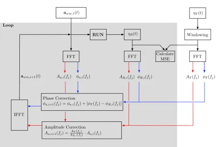
2.3. Calibration procedure 141

The source acceleration,awm(t), is calibrated, using a standard spectral analysis method, based on

142

work presented in [?], to produce a target wave series at a desired position within the NWT. Figure?? 143

shows a schematic of the calibration procedure, which comprises the following steps:

1. Define target wave series at desired NWT location,ηT(t), with a signal lengthL andN samples

145

2. Perform a Fast Fourier Transform (FFT) on ηT(t), to obtain the amplitudes, AT(fj), and phase

146

components,φT(fj), for each frequency component,fj, withj={1, 2, ...,N2 }, where f1= _L0,f2= 147

1

L, ...,fN = 2NL − 1

L 148

3. Generate an initial time series for the wavemaker source term,awm,1(t)(can be chosen randomly or 149

informed byηT(t))

150

4. Perform a FFT onawm,1(t), to obtain the amplitudes,Aa,1(fj), and phase components,φa,1(fj), for

151

each frequency component of the input source term

152

5. Run simulation, for iterationi, using the wavemaker source termawm,i(t), and measure the resulting

153

free surface elevation at the chosen NWT location,ηR,i(t)

154

6. Perform a FFT onηR,i(t), to obtain the amplitudes,AR,i(fj), and phase components,φR,i(fj), for each

155

frequency component of the generated wave series

156

7. Calculate the new amplitudes for each frequency component of the input source term,Aa,i+1(fj),

157

by scaling the previous amplitudes,Aa,i(fj), with the ratio of target surface elevation amplitude,

158

AT(fj), and the generated surface elevation amplitude from the previous run,AR,i(fj):

159

• Aa,i+1(fj) = AT(fj)

A_R,i(f_j)Aa,i(fj) 160

8. Calculate the new phase components,φa,i+1(fj), by summingφa,i(fj)with the difference between

161

the target elevation phase,φT(fj), and the measured surface elevation phase from the previous run,

162

φR,i(fj):

163

• φa,i+1(fj) =φa,i(fj) +

φT(fj)−φR,i(fj)

164

9. Generate the new time series for the wavemaker source term,awm,i+1(t), by performing an Inverse 165

Fourier Transform onAa,i+1(fj)andφa,i+1(fj)

166

10. Repeat steps 5 - 9 until either a maximum number of iterations, or a threshold for the mean-squared

167

error (MSE) between the target and resulting surface elevation, is reached.

168

It should be noted, that although the method is based on the work described by [?], we have further

169

simplified it. Instead of evaluating the phase-shift caused by the distance between the wavemaker and the

170

point of interest, which would require the use of some wave theory to find the wavenumberk, we directly

171

adjust the phase between wavemaker and target (Step 8).

172

2.4. Calibration procedure for regular waves 173

The calibration method detailed above might fail to resolve the single peak in frequency domain for

174

short time traces of regular waves. At the same time, in regular waves the phase of the wave is generally

175

not of interest, allowing for a simplification of the calibration . [? ? ?] used the same solver formulation

176

and simply tuned the amplitude of an oscillating source to create monochromatic waves of a desired

177

height. The following calibration method is used for regular waves:

178

1. The source term is set to oscillate in horizontal direction with the desired wave frequency.

179

2. The amplitudeAa,iis initialised with an arbitrary value.

180

3. After the initial, and each subsequent run, the surface elevation is analysed in time domain. The

181

mean is removed from the surface elevation. Mean wave heightHR,iis then obtained as the difference

182

between the mean of the positive and mean of the negative peaks.

183

4. A new wave maker amplitudeAa,i+1is obtained by linearly scaling the previous value with the ratio 184

of targetHTand result wave heightHRas followsAa,i+1= HH_R,iT Aa,i

185

Steps 3 and 4 are repeated until the desired wave height is achieved.

ηT(t)

FFT

AT(fj) φT(fj)

FFT

Aa,i(fj) φa,i(fj)

RUN ηR(t)

FFT

AR,i(fj) φR,i(fj)

Calculate MSE

Phase Correction

φa,i+1(fj) =φa,i(fj) + [φT(fj)−φR,i(fj)]

IFFT Loop

Windowing

awm,i+1(t)

awm,1(t)

Amplitude Correction Aa,i+1(fj) =AAR,iT(f(fjj))·Aa,i(fj)

Figure 1.Schematic of the Calibration Method

3. Case study 187

A case study is now presented with two main objectives, firstly to demonstrate the capabilities of

188

the impulse wavemaker and the self-calibration procedure in producing any realistic deep or shallow

189

water wave series at a specified location in a wave tank. The second objective is to provide guidance on

190

the selection of the wavemaker source region, by investigating the effect that the size and position of the

191

source region has on the resulting waves. It might be expected that a very long source area will decrease

192

accuracy, whereas a very short source region will require very large velocity components to create a target

193

wave. For the shallow water impulse wavemaker in [? ], a source length of about a quarter to half a

194

wavelength is recommended. In shallow water, the entire water column, from the sea floor up to the water

195

surface, performs an oscillating motion, whereas in deep water only part of the water column is affected

196

and the wave motion does not extend to the sea floor. It is thus an interesting question how to choose the

197

length and depth of the source region to achieve optimal results in deep, as well as shallow, water.

198

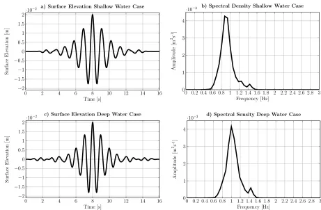
3.1. Target waves 199

The case study considers two types of target waves, multi-frequency and regular waves, to

200

demonstrate the calibration procedures outlined in Sections??and??, respectively.

201

3.1.1. Multi-frequency wave packet

202

To demonstrate the ability of the impulse wavemaker, the case study creates a unidirectional

203

multi-frequency wave packet at a specified location in the NWT. The wave packet considered is a realisation

204

of the NewWave formulation as presented in [?]. A NewWave wave packet comprises a summation of all

the frequency components of a given spectrum, such that the largest amplitude wave crest is created in the

206

temporal centre of the packet. The governing equations for the surface elevation,ηT(t), and amplitude of

207

each wave component,ak, withk=1, ...,K, are given in Eq. (??) and (??), respectively:

208

ηT(t) =

K

∑

k=1

akcos[kk(x−x0)−ωk(t−t0)] (4)

ak=A0 S(fk)∆f

∑Kk S(fk)∆f

(5)

In Eq. (??),x0 represents the spatial focal location andt0the temporal focal instant. In Eq. (??), 209

S(f)is the spectral density and∆f the frequency step.A0represents the amplitude of the largest wave 210

crest. For this case study,A0=0.02 m,∆f =0.1 s−1, andTp=1.1 s for the shallow case, contrasted with

211

Tp=0.977 s for the deep water case. The different peak periods are chosen such that the peak wavelength,

212

λpof 1.48 m remains identical across cases, yieldingkhparameters of 1.06 for the shallow and 3.13 for the

213

deep water case.

214

Although the parameters used in this case study are somewhat arbitrarily chosen, wave packets

215

are generally well suited for testing the calibration of amplitudes and phases of different frequency

216

components [? ], and are also of practical relevance in industrial applications [? ]. Time traces for the

217

surface elevationη(t), and plots of the spectra densityS(f)for the shallow and deep water case, are shown 218

in Fig.??.

219

0 0.2 0.4 0.6 0.8 1 1.2 1.4 1.6 1.8 2 2.2 2.4 2.6 2.8 3 0

1 2 3 4

·10−3

Frequency [Hz]

Amplitude

[m

2-1s

]

d) Spectral Sensity Deep Water Case

0 2 4 6 8 10 12 14 16

−2 −1.5 −1 −0.5 0 0.5 1 1.5

2·10

−2

Time [s]

Surface

Elev

ation

[m]

c) Surface Elevation Deep Water Case

0 2 4 6 8 10 12 14 16

−2 −1.5 −1 −0.5 0 0.5 1 1.5

2·10

−2

Time [s]

Surface

Elev

ation

[m]

a) Surface Elevation Shallow Water Case

0 0.2 0.4 0.6 0.8 1 1.2 1.4 1.6 1.8 2 2.2 2.4 2.6 2.8 3 0

1 2 3 4

·10−3

Frequency [Hz]

Amplitude

[m

2-1s

]

b) Spectral Density Shallow Water Case

3.1.2. Regular waves

220

Two cases demonstrating the creation of regular waves in shallow and deep water are presented.

221

The target wave height was set to 0.037mand the period to 1.1sfor the shallow water case and 0.977s 222

for the deep water case, replicating the peak frequency and maximum wave height of the corresponding

223

wave packets described in Section??. If not mentioned specifically the settings found to be suitable for the

224

corresponding wave packets have been used for the setup of these regular wave cases.

225

3.2. Source region 226

A rectangular shaped source region is used for all simulations, whose length,L, and height,H, are

227

varied to investigate the effect of the source region size on the wave maker performance. Additionally, to

228

investigate the effect of the position of the wavemaker within the water column, the depth of the source

229

region is varied.

230

3.3. Simulation platform 231

The NWT implementation for this case study is based on theinterFoamsolver from the OpenFOAM

232

toolbox. TheinterFoamsolver uses a volume of fluid (VOF) approach for modelling the two different fluid

233

phases, air and water, in order to capture and track and the free surface. More details on this solver can be

234

found in [?]. Although the case study employs OpenFOAM as the CFD solver, the method can easily be

235

applied to any CFD software that allows user coding. For example, [?] implements the shallow water

236

impulse source wavemaker in ANSYS Fluent, using its user-defined functions capability.

237

The calibration function was implemented in the free scientific programming software, GNU Octave

238

[?]. This results in all of the software utilised in this case study being opensource or free. The source code

239

for the case study set-up and implementation has been shared by the authors on the CCP-WSI repository

240

[?], allowing anyone to easily access and utilise the developed impulse source wavemaker.

241

3.4. Numerical wave tank set-up 242

Since the case study considers a unidirectional input wave, a two-dimensional (2D) NWT is

243

implemented to simplify the set-up and reduce computational overheads. The NWT set-up is described

244

below, detailing the geometry, boundary conditions, mesh and calibration of the absorption beach.

245

3.4.1. Geometry

246

The NWT geometry is depicted in Figure??. The depth of the NWT is set to 0.25 m for the shallow

247

water case, and 0.74 m for the deep water case. The target location for the input wave packet is located 3 m

248

downwave from the centre of the wavemaker source region. Two absorption beaches are then located at

249

1.5 m upwave and 5.5 m downwave from the source centre.

250

3.4.2. Boundary conditions

251

The front and back faces of the NWT, lying in thex−zplane, are set toempty, indicating a 2D

252

simulation. The bottom, left and right boundaries are set to a wall. The top boundary is set to atmospheric

253

inlet/outlet condition.

254

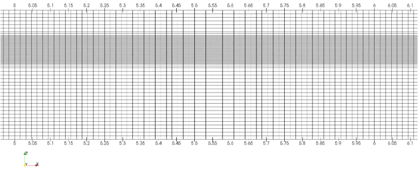
3.4.3. Mesh

255

The mesh is depicted in Figure??. The mesh is one cell thick in theydirection, for implementation of

256

the 2D simulation. Mesh refinement has been employed in the interface region leading to a cell size of 8

257

13m

0.36m d

beach beach

lbeach

source region

H

L wave probe

3m

Figure 3.Schematic of the NWT including the main dimensions. For the shallow water cases the water depthdis set to 0.25m, for the deep water case is 0.74m

these sizes. Adjustable time stepping, based on a maximum allowable Courant number of 0.9, is used in

259

all simulations.

260

3.4.4. Calibration of the absorption beach

261

[? ] recently published a method based on analytical theory to find the ideal magnitude of the

262

damping parametersandfor monochromatic waves. In the future it will thus be possible to set the ideal

263

damping parameters prior to each simulation. Herein, a parameter study is performed to investigate

264

the absorption performance for the wave packet. Three different pairs oflbeachandsandMaxwere tested

265

for the shallow water case, i.e. lbeach =λpandsandMax =5;lbeach = λpandsandMax =7,lbeach = 2λp

266

andsandMax =6. The first test, usingsandMax =5s−1andlbeach=λp, yielded a reflection coefficient of

267

3.5%, with reflection evaluated using the method described in [?]. IncreasingsandMax to 7s−1results in

268

a reflection coefficient of 2.5%; usingsandMax =6s−1andlbeach =2λpreduced the reflection coefficient

269

significantly to 0.2%. The latter beach configuration was then used in all subsequent cases. While even

270

the first configuration, with a resulting reflection coefficient of 3.5%, is better than most experimental

271

facilities [?] and many numerical methods, it highlights the flexibility of the approach. Larger beaches

272

will invariably come with a greater computational cost but, for cases where very low reflection over a

273

larger frequency range is required, they seem the only viable method. Fig??shows the definition of the

274

dissipation parameter along the tank as used in the simulations.

Figure 5.Gradually increasing damping factorsand. The grading depends on the location, with no damping (blue colour code) in the centre of the wave tank and highest damping (red colour code) at the far field boundaries

275

3.5. Source region test cases 276

120 muti-freqeuncy wave packet experiments were run in total, for 90 shallow water cases and 30 deep

277

water cases, with varying source region layouts investigated. For the shallow water cases, simulations

278

were run with the source region progressively centred at a third, a half, and two thirds of the water

279

depth. For deep water cases, the centre of the source region is located at a depth of λp₄, or half the

280

water depth. For each different source centre location, 30 experiments were run with varying source

281

length region,L, of 0.125λp, 0.25λp, 0.5λp, 1λp, 1.25λpand varying height of the source region, H, of

282

0.125d, 0.25d, 0.5d, 0.75d, 1dand 1.25d.

The performance of the various source region layouts is evaluated as the MSE between the target surface elevation,ηT, and the achieved result,ηR:

MSE= 1 K

K

∑

l

(ηT,l−ηR,l)2, (6)

whereKis the total number of time steps in the simulation.

284

4. Results and Discussion 285

In this section the case study results are presented and discussed. First, an example result from a

286

single experiment (deep water case with source height of λp₈ and source length of 1₄λp) is presented in

287

Section??. The complete set of the results from all the shallow and deep water experiments are summarised

288

in Sections??and??, respectively. Application of the simplified calibration method for regular waves is

289

discussed in??.

290

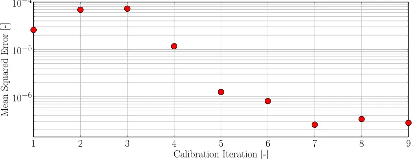
4.1. Example result 291

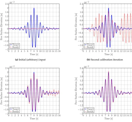
Figure??displays an example of the typical decrease in MSE for increasing calibration iterations

292

during an experiment. Note the evolution is non-monotonic, which is explained by Figure??, showing

293

the corresponding surface elevation time traces from a selection of these calibration iterations. The first

294

iteration is initialised with random input of small amplitude, and the resulting surface elevation is almost

295

zero and the MSE of 3×10−5, is large. The second iteration yields several waves with similar amplitude

296

and frequency to the target wave packet, but out of phase, and the resulting MSE almost doubles. The

297

fourth and fifth iterations decrease the MSE by orders of magnitude to 1×10−5and 1×10−6. The main

298

peak of the wave packet is now already very well resolved and most of the error stems from some small

299

high frequency waves after 11 s. Further iterations decrease the MSE to about 3×10−7, agreement is now

300

even good for the small ripples after 11 s. For all the results presented Sections??and??, 9 calibration

301

iterations are used.

302

1 2 3 4 5 6 7 8 9

10−6 10−5 10−4

Calibration Iteration [-]

Mean

Squared

Error

[-]

0 1 2 3 4 5 6 7 8 9 10 11 12 13 14 15 16 −2

−1.6 −1.2 −0.8 −0.4 0 0.4 0.8 1.2 1.6 2 2.4·10−2

Time [s] F ree S urface Elev ation [m] Target Result

(a)Initial (arbitrary) input

0 1 2 3 4 5 6 7 8 9 10 11 12 13 14 15 16 −2

−1.6 −1.2 −0.8 −0.4 0 0.4 0.8 1.2 1.6 2 2.4·10−2

Time [s] F ree S urface Elev ation [m] Target Result

(b)Second calibration iteration

0 1 2 3 4 5 6 7 8 9 10 11 12 13 14 15 16 −2

−1.6 −1.2 −0.8 −0.4 0 0.4 0.8 1.2 1.6 2 2.4·10−2

Time [s] F ree S urface Elev ation [m] Target Result

(c)5th calibration iteration

0 1 2 3 4 5 6 7 8 9 10 11 12 13 14 15 16 −2

−1.6 −1.2 −0.8 −0.4 0 0.4 0.8 1.2 1.6 2 2.4·10−2

Time [s] F ree S urface Elev ation [m] Target Result

(d)Final calibration iteration

Figure 7.Example of the target and resulting surface elevation, at different calibration iterations, for the same case as Fig.??

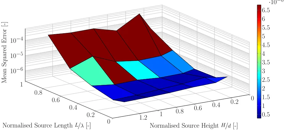
4.2. Shallow water waves 303

The results from the shallow water experiments are summarised in Figures??,??and??, for the cases

304

with the center of the source region at one third, one half and two thirds of the water depth, respectively.

305

The results show that decreasing the length of the source region, from 1λpto 0.3λpor less, reduces the

306

MSE by over two orders of magnitude. In contrast, the height of the source region is seen to have a much

307

smaller influence on the wavemaker performance, with best results obtained when the source region spans

308

over the entire water depth. Overall, the smallest MSE occurs for the experiment with the source region

309

centred at half the water depth, the source length of 0.25λp, and a source height of 1.25 times the water

310

depth,

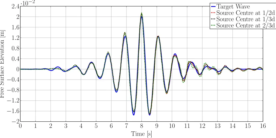
Figure??shows the target wave time series and the results of the experiments which produced the

312

best results for the three different source centre depths. Variations between simulations are minimal.

313

The centre of the wave packet is very well reproduced around its peak and the surrounding crests and

314

troughs, with the main discrepancies occurring at the beginning and the end of the wave packet, with the

315

CFD simulations presenting small amplitude ripples when the target wave is already reaching still water

316

conditions.

317

0

0

.

2

0

.

4

0

.

6

0

.

8

1

0

0

.

2

0

.

4

0

.

6

0

.

8

1

1

.

2

10

10

10

Normalised Source Length

_/

[-]

Normalised Source Height

_/

[-]

Mean

Squared

Error

[-]

0

.

5

1

1

.

5

2

2

.

5

3

3

.

5

4

4

.

5

5

5

.

5

6

6

.

5

·

10

Figure 8.Shallow water case - Source centre atd₃: Minimal error (4.5×10−7_{) for source height of 1dand}

source length1₄λp

0

0

.

2

0

.

4

0

.

6

0

.

8

1

0

0

.

2

0

.

4

0

.

6

0

.

8

1

1

.

2

10

10

10

Normalised Source Length

_/

[-]

Normalised Source Height

_/

[-]

Mean

Squared

Error

[-]

0

.

5

1

1

.

5

2

2

.

5

3

3

.

5

4

4

.

5

5

5

.

5

6

6

.

5

·

10

0

0

.

2

0

.

4

0

.

6

0

.

8

1

0

0

.

2

0

.

4

0

.

6

0

.

8

1

1

.

2

10

10

10

Normalised Source Length

_/

[-]

Normalised Source Height

_/

[-]

Mean

Squared

Error

[-]

0

.

5

1

1

.

5

2

2

.

5

3

3

.

5

4

4

.

5

5

5

.

5

6

6

.

5

·

10

Figure 10.Shallow water case - Source centre at2₃d: Minimal error (5.9×10−7) for source height of 1.25d

and source length1₂λp

0

1

2

3

4

5

6

7

8

9

10

11

12

13

14

15

16

−

2

−

1

.

6

−

1

.

2

−

0

.

8

−

0

.

4

0

0

.

4

0

.

8

1

.

2

1

.

6

2

2

.

4

·

10

Time [s]

F

ree

S

urface

Elev

ation

[m]

Target Wave

Source Centre at 1/2d

Source Centre at 1/3d

Source Centre at 2/3d

Figure 11.Surface elevation time series for shallow water experiments which produced the best results for the three different source centre locations

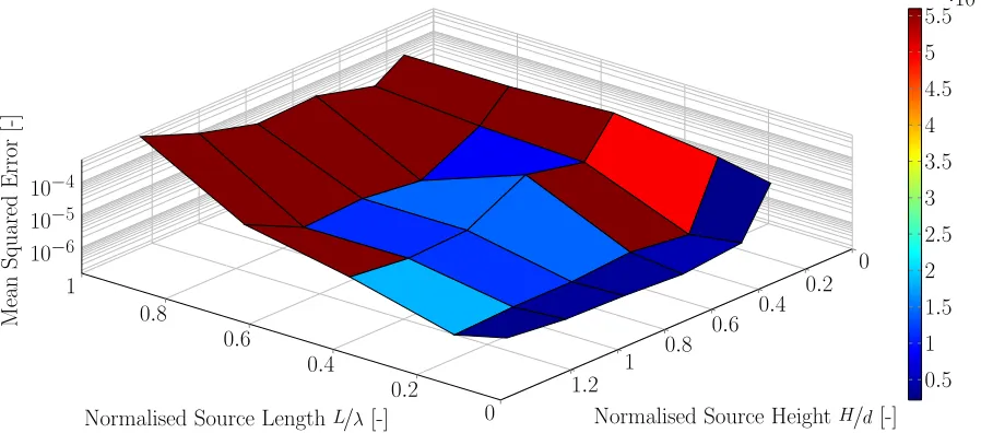
4.3. Deep water waves 318

Deep water waves only affect the water column up to a depth of half a wave length, it thus seems

319

more appropriate to base the vertical position of the source region on that parameter. Because the source

320

center position had little influence in the shallow water cases presented earlier, test cases were only run for

321

varying source heights and lengths, with the source centre position fixed atλp/4.

Figure??shows the results from the deep water experiments. The minimum error is 2.8×10−7for a

323

source length of 0.25λpand height of 0.25 times the water depth, which is somewhat less than the best

324

shallow water case. A wide range of source heights yields good results; only for small values of source

325

heights, where the source region does not reach the surface, does the error increase significantly.

326

0 0.2

0.4 0.6

0.8 1

0 0.2 0.4 0.6 0.8 1 1.2 10−6

10−5 10−4

Normalised Source LengthL_/λ[-] Normalised Source HeightH_/d[-]

Mean

Squared

Error

[-]

0.5 1 1.5 2 2.5 3 3.5 4 4.5 5 5.5·10

−6

Figure 12.Deep water case: Minimal error (5·10−4_{) for source height of}λp

8 and length14λp

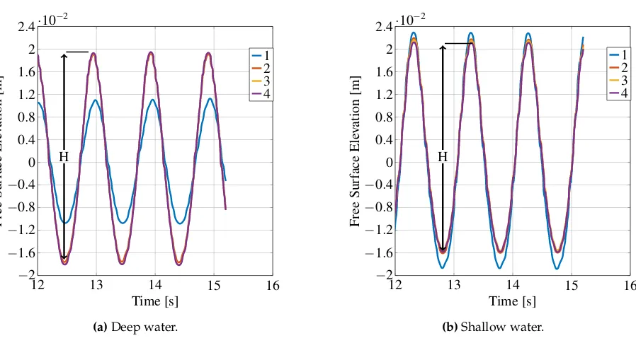
4.4. Regular waves 327

Figure??shows the surface elevation during the first four calibration steps for deep and shallow

328

water waves. In both cases the results converged rapidly, after the second iteration the results are almost

329

identical for subsequent runs. Figure??shows the absolute difference between target wave height and

330

the current value. For the second iteration errors are already within the millimetre range and decrease

331

almost another order of magnitude in the third iteration, which can be deemed sufficient for any practical

332

application.

12 13 14 15 16

−2 −1.6 −1.2 −0.8 −0.4

0 0.4 0.8 1.2 1.6 2 2.4·10−2

H

Time [s]

Free

Surf

ace

Ele

vation

[m]

1 2 3 4

(a)Deep water.

12 13 14 15 16

−2 −1.6 −1.2 −0.8 −0.4

0 0.4 0.8 1.2 1.6 2 2.4·10−2

H

Time [s]

Free

Surf

ace

Ele

vation

[m]

1 2 3 4

(b)Shallow water.

Figure 13.Surface elevation time series for regular waves. Numbers indicate the calibration iteration.

5. Conclusion 334

A NWM, based on the impulse source method, was implemented in the OpenFOAM framework.

335

In combination with a calibration procedure, complex irregular wave patterns can be recreated in deep

336

and shallow water, using an impulse source term acting in the horizontal direction. While the simple

337

formulation of the source term facilitates implementation in the flow solver, the calibration procedure

338

ensures that the target wave is created at the desired position and time in the NWT. Furthermore,

339

reflection analysis demonstrates the ability of the numerical beach to achieve arbitrarily low reflection

340

from boundaries and transparency of the wavemaker region. In the future, the work of [?] will allow to

341

set the ideal beach parameters without the need to run parameter or calibration studies.

342

1 2 3 4

10−5 10−4 10−3 10−2 10−1 100

Calibration Iteration [-]

Error

[-]

Deep Shallow

Parameter sensitivity studies, investigating the effect of the shape and position of the wavemaker

343

region, show that good results can be achieved over a wide range of parameters. For deep and shallow

344

water, a wavemaker region length of less than a quarter of a wave length is suitable, which is less than

345

recommended in previous work [?], and might enable the use of smaller computational domains. The

346

vertical position of the centre of the wavemaker has overall little effect in shallow water conditions and

347

good results were achieved if it was placed at half the water depth. For deep water cases, good results

348

were obtained with the centre of the wavemaker at a quarter of a wave length below the surface. Even

349

when starting from a poor initial parameter specification, the method is shown to converge to an accurate

350

solution within a few iterations.

351

For monochromatic or regular waves, a simplified calibration method can be used. Tests show that

352

the the amplitude can typically be found within four iterations.

353

Although the calibration method is standard in experimental test facilities, it can be expected to

354

become inaccurate in higher order sea states. Improvements should be explored to take into account

355

non-linear effects. A possible way forward might be neural networks of arbitrary complexity as described

356

by [?].

357

Acknowledgements 358

This paper is based upon work supported by Science Foundation Ireland under Grant No. 13/IA/1886.

359

Pál Schmitt’s Ph.D. was made possible by an EPSRC Industrial Case Studentship 2008/09 Voucher 08002614

360

with industrial sponsorship from Aquamarine Power Ltd.

361