Trigonometric Cubic B-spline Collocation Method
for Solitons of the Klein-Gordon Equation
Alper Korkmaz
1,*, Ozlem Ersoy
2and Idiris Dag
31
Department of Mathematics, C¸ ankırı Karatekin University, 18200 C¸ ankırı, Turkey
2
Department of Mathematics & Computer, Eskisehir Osmangazi University, 26480 Eskisehir, Turkey;
3
Department of Computer Engineering, Eskisehir Osmangazi University, 26480 Eskisehir, Turkey;
*
Correspondence: [email protected]December 2, 2016
Abstract
In the present study, we derive a new B-spline technique namely trigono-metric B-spline collocation algorithm to solve some initial boundary value problems for the nonlinear Klein-Gordon equation. In order to carry out the time integration with Crank-Nicolson implicit method, the order of the equation is reduced to give a coupled system of nonlinear partial differen-tial equations. The collocation approximation based on trigonometric cubic B-splines for spatial discretization is followed by the linearization of the non-linear term. The efficiency and accuracy of the present method are validated by measuring the error between the numerical and analytical solutions when exist. The conservation laws representing momentum and energy are also computed for all problems.
Keywords: Klein-Gordon equation; trigonometric cubic B-spline; collocation; soli-ton; wave motion; conservation laws
AMS2010: 65M70.
1
Introduction
Consider the Klein-Gordon equation of the form
whereu=u(x, t),P0(u) is some reasonable nonlinear function ofu [1]. P(u) does not include the derivatives ofuand can be chosen as the potential energy in many studies. The equation was derived by Klein and Gordon as a relativistic equation for a charged particle in an electromagnetic field [2]. Some particular forms of the equation are used as model for many fields such as Josephson junction transmission lines, dislocation in crystals, the propagation in ferromagnetic materials of waves carrying rotations of the direction of magnetization, laser pulses in two state me-dia, torsional waves propagating down a stretched wire in a pendula system, etc. According to Detweiler, The Klein-Gordon equation can also be useful to analyze the rotating black holes [3]. The equation can be constructed geometrically by the invariance of the scalar curvature with some particular gauge and coordinate transformations [4]. The scattering field theory for the Klein-Gordon equation was developed by following the usual procedure of a first order equivalent equation in the vector valued functions Hilbert space equipped with a finite energy norm [5]. The spectral and scattering theory based on the eigenfunction expansion was also derived for the Klein-Gordon equation in the static external field [6].
Besides, its applications in many fields summarized above, the Klein-Gordon equa-tion with cubic nonlinear term can be converted to the nonlinear Schr¨ı¿12dinger equation with cubic nonlinearity [7]. However, the sign of the cubic term is the key for the existence of the envelope soliton or hole solutions owing to the fact that the stability of the nonlinear Klein-Gordon equation depends on it [8]. The existence of compactonlike kink solutions of the Klein-Gordon equation was discussed by investigating the existence and stability of compact entities numeri-cally [9]. Kim and Hong [10] determine the solitary wave solutions including the powers of sech and tanh functions of the generalized Reaction Duffing equations, which is a generalization of some nonlinear equations, the Landau-Ginzburg-Higgs, the Φ4 and the Klein-Gordon equation with cubic nonlinear term, by the auxiliary
ordi-nary differential equation satisfied by a particular homogenous function can lead to the nonlinear Klein-gordon equation. Interaction of solitons of the Klein-Gordon equation was investigated in different aspects in various numerical studies [17–19]. Different from many analytical studies summarized above, various numerical al-gorithms have also been developed to obtain solutions of different problems for the Klein-Gordon equation. The central second difference approximation of the finite difference method was implemented to the nonlinear Klein-Gordon equation to solve some initial boundary value problems to show the bounded solutions as t → ∞ [20]. The degree of the power term directly affects the amplitude and the number of oscillations. Jim¨ı¿12nez and V¨ı¿12zquez [21] compared the results obtained by four explicit finite difference schemes and concluded that the energy conserving scheme is the most convenient technique to integrate the Klein-Gordon equation to examine the long time behaviour. Some initial boundary value prob-lems for the inhomogenous form of the Klein-Gordon equation with various degreed nonlinear terms were also solved by the thin plate splines radial basis functions collocation method [22]. Multiquadric Quasi-interpolation technique is another ef-ficient technique to determine the solutions of the equation [23]. Cao and Guo [24] proposed the Fourier collocation method to solve a periodic problem by investi-gating its stability and convergence properties.
Classical polynomial cubic B-spline collocation on a uniform mesh distribution was implemented to the some problems derived on the nonlinear Klein-Gordon equa-tion [25]. Zahra et al. [26] derived an uncondiequa-tionally stable collocaequa-tion method based on the cubic B-splines for the solution of an initial boundary value problem. Different from these studies, we suggest a new collocation method based on non polynomial cubic B-spline, namely trigonometric cubic B-splines, to solve some initial boundary value problems for the nonlinear Klein-Gordon equation of the particular form
utt−uxx =ε1u+ε2u3 (2)
where ε1 and ε2 are nonzero constants. Assuming v =ut reduces the order of the equation to lead a coupled system of nonlinear partial differential equations
vt =uxx+ε1u+ε2u3
ut=v
(3)
The complementary conditions describing the associated problem are
u(x,0) =f(x), a≤x≤b ux(a, t) =ux(b, t) = 0, t >0
vx(a, t) =vx(b, t) = 0, t >0
(4)
2
Numerical Approach and Construction of the
Algorithm
The discretization of the system (3) in time by usual forward finite difference and by Crank-Nicolson method yields
vn+1−vn
∆t =
un+1 xx +unxx
2 +ε1
un+1+un
2 +ε2
(u3)n+1+ (u3)n 2
un+1−un
∆t =
vn+1+vn 2
(5)
where un+1 =u(x,(n+ 1)∆t) represents the solution at the (n+ 1)th. time level. Heretn+1 =tn+ ∆t, and ∆t is the time step, superscripts denote the time levels. Linearization of the term (u3)n+1 in (5) as
(u3)n+1 = 3un+1(u2)n−2(u3)n
gives the time-integrated Klein-Gordon equation
vn+1−vn
∆t =
un+1 xx +unxx
2 +ε1
un+1+un
2 +ε2
3un+1(u2)n−(u3)n 2
un+1−un
∆t =
vn+1+vn 2
(6)
LetGbe a uniform grid distribution of the artificial problem interval [a, b] defined as G : a = x1 < x2 < . . . < xN = b, h =xi −xi−1, i = 2,3, ..., N. Different from
the other B-splines [27–30], the trigonometric cubic B-splines with nonzero values in this interval for this grid distribution are defined as
Ci(x) = 1 θ
ω3(xi−2) , [xi−2, xi−1]
ω(xi−2)(ω(xi−2)φ(xi) +ω(xi−1)φ(xi+1)) +φ(xi+2)ω2(xi−1) , [xi−1, xi]
ω(xi−2)φ2(xi+1) +φ(xi+2)(ω(xi−1)φ(xi+1) +ω(xi)φ(xi+2)) , [xi, xi+1]
φ3(xi+2) , [xi+1, xi+2]
0 , otherwise
,
i= 0,1, . . . , N + 1
(7) where ω(xi) = sinx−2xi, φ(xi) = sinxi2−x, θ = sinh2sinhsin32h [31]. The set
{C0(x), C1(x), ..., CN+1(x)} forms a basis for the functions defined in the
inter-val [a, b].
EachCi(x) is twice continuously differentiable and the nonzero values ofCi(x), C
0
Table 1: Values ofCi(x) and its derivatives at knots
Ci(xi) Ci0(xi) Ci00(xi)
xi−2 0 0 0
xi−1 sin2(h2) csc (h) csc(32h) 34csc(32h)
3(1+3 cos(h)) csc2(h
2) 16[2 cos(h2)+cos(32h)]
xi 1+2 cos(2 h) 0
−3 cot2(32h) 2+4 cos(h)
xi+1 sin2(h2) csc (h) csc(32h) −34csc(32h)
3(1+3 cos(h)) csc2(h
2) 16[2 cos(h
2)+cos( 3h
2)]
xi+2 0 0 0
LetU(x, t) andV(x, t) be the approximate solutions tou(x, t) andv(x, t), respec-tively, defined as
U(x, t) = N+1
X
i=−1
δiCi(x),
V(x, t) = N+1
X
i=−1
φiCi(x)
(8)
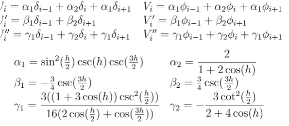
in which δi and φi are the time dependent parameters. The nodal values of the approximate solutionsU andV and their first and second derivatives can be found from the (8) as
Ui =α1δi−1 +α2δi+α1δi+1
Ui0 =β1δi−1+β2δi+1
Ui00 =γ1δi−1+γ2δi+γ1δi+1
Vi =α1φi−1+α2φi+α1φi+1
Vi0 =β1φi−1+β2φi+1
Vi00 =γ1φi−1+γ2φi+γ1φi+1
(9)
α1 = sin2(h2) csc(h) csc(32h) α2 =
2 1 + 2 cos(h) β1 =−34csc(32h) β2 = 34csc(32h)
γ1 =
3((1 + 3 cos(h)) csc2(h2))
16(2 cos(h2) + cos(32h)) γ2 =−
3 cot2(h2) 2 + 4 cos(h)
where Ui and Vi represent U(xi) and V(xi), respectively.
Substituting the approximate solutions (8) and their derivatives into (6) and re-arranging the resulting equations by using nodal values of trigonometric B-spline functions gives the iterative system
κm1δmn+1−1 +κm2φnm+1−1+κm3δmn+1+κm4φnm+1+κm1δmn+1+1+κm2φnm+1+1 (10)
= κm5δmn−1 +κm2φnm−1+κm6δmn +κm4φnm+κm5δmn+1+κm2φnm+1
κm2δmn+1−1 +κm7φnm+1−1+κm4δmn+1+κm8φnm+1+κm2δmn+1+1+κm7φnm+1+1 (11)
The coefficients of equation system (10) and (11) for KGE equation can be deter-mined as follow
κm1 = (−3ε2K2−ε1)α1−γ1
κm2 =
2 ∆tα1
κm3 = (−3ε2K2−ε1)α2−γ2
κm4 =
2 ∆tα2
κm5 = (ε1−ε2K2)α1+γ1
κm6 = (ε1−ε2K2)α2+γ2
κm7 =−α1
κm8 =−α2
where
K =α1δin−1+α2δin+α1δni+1
The system (10) and (11) can be converted the following system in the matrix form
Adn+1 =Bdn (12)
where A=
κm1 κm2 κm3 κm4 κm1 κm2
κm2 κm7 κm4 κm8 κm2 κm7
κm1 κm2 κm3 κm4 κm1 κm2
κm2 κm7 κm4 κm8 κm2 κm7
. .. ... ... ... ... ... κm1 κm2 κm3 κm4 κm1 κm2
κm2 κm7 κm4 κm8 κm2 κm7
and B =
κm5 κm2 κm6 κm4 κm5 κm2
κm2 −κm7 κm4 −κm8 κm2 −κm7
κm5 κm2 κm6 κm4 κm5 κm2
κm2 −κm7 κm4 −κm8 κm2 −κm7
. .. . .. . .. . .. . .. . ..
κm5 κm2 κm6 κm4 κm5 κm2
κm2 −κm7 κm4 −κm8 κm2 −κm7
The system (12) consists of 2N+ 2 linear equations in 2N+ 6 unknown parameters dn+1 = (δ−n+11 , φn−+11 , δ0n+1, φn0+1. . . , δnN+1+1, φnN+1+1). A unique solution of the system is dependent on the equal number of equations and parameters. Imposing the boundary conditions
gives a chance to reduce the number of parameters by generating relations between the parameters
δ−1 =δ1, φ−1 =φ1, δN−1 =δN+1, φN−1 =φN+1
Elimination of the parametersδ−1, φ−1, δN+1, φN+1 provides a solvable system
hav-ing 2N + 2 linear equations with 2N + 2 unknown parameters. In the study, we solved this system by using adapted Thomas algorithm for the systems having six-banded coefficient matrices.
In order to initialize the iteration algorithm, we need the initial parameter vector d0. Assuming d0
1 = (δ0−1, δ00, ..δN0, δN0+1), d02 = (φ0−1, φ00, ..φ0N, φ0N+1) are the
compo-nents of the initial vector d0 of the iteration, we eliminate the parameters using the equalities
Ux(a,0) = 0 =δ0−1−δ 0 1,
Ux(xi,0) = δi0−1 −δ 0
i+1 =Ux(xi,0), i= 1, ..., N −1
Ux(b,0) = 0 =δ0N−1−δ 0 N+1,
Vx(a,0) = 0 =φ0−1−φ 0 1
Vx(xi,0) = φ0i−1−φ 0
i+1 =Vx(xi,0), i= 1, ..., N −1
Vx(b,0) = 0 =φ0N−1−φ0N+1
(13)
to be able to initalize the iteration (12).
3
Numerical Illustrations
The validity and efficiency of the proposed method are checked by measuring the error between the numerical and the analytical solutions when exist using the discrete maximum error norms defined as
L∞(t) = |u(x, t)−U(x, t)|∞= max
i |u(xi, t)−U(xi, t)|
at the time t.
The conservation laws computed by the numerical results representing energy(E) and momentum(P) [1, 2, 32]
E = 1 2
∞
Z
−∞
u2t +u2x−ε1u2−
1 2ε2u
4
dx
P =
∞
Z
−∞
uxutdx
for the nonlinear Klein-Gordon can also be also good indicators of the validity of the method even when the analytical solutions do not exist. The absolute relative changes C(Et) and C(Pt) of conservation lawsE and P are defined as
C(Et) =
Et−E0
E0
C(Pt) =
Pt−P0
P0
(15)
where E0 and P0 are initial values of energy and momentum, respectively, as Et and Pt are the computed values of these two laws at the time t.
3.1
sech-type Single Solitary Wave
The sech-type single solitary wave solution for the parameters ε1 = 2, ε2 = −1
choice in the Klein-Gordon equation is given as
u(x, t) = 2 sech (√2{sinh (1)}x− {cosh (1)}t) (16)
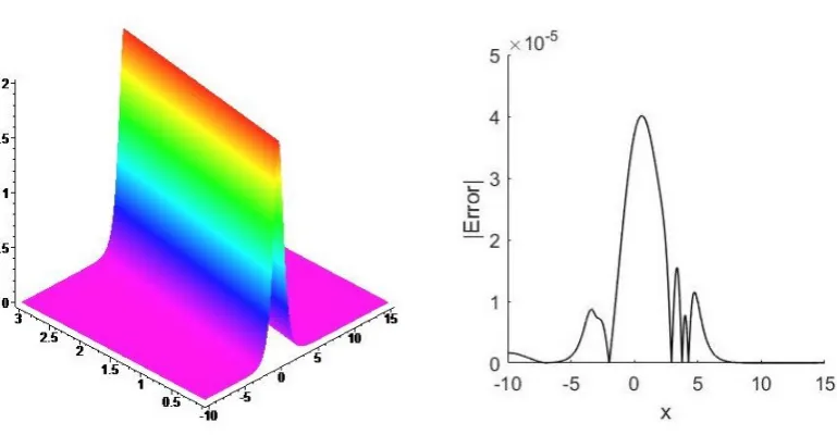
where sinh and cosh are known hyperbolic functions [33]. This solution represents a traveling wave of amplitude 2 whose peak is positioned atx= 0 initially. As time passes, the wave propagates to the right along thex−axis. In order to accomplish the numerical simulation, the articifical problem interval is considered as [−10,15]. The initial condition is adapted from the analytical solution by substitutingt = 0 in the solution. The algorithm is run for various time and space step lengths up to the terminating time t = 3. The propagation of the single solitary wave is simulated in Fig 1(a). The numerical results seem in a good agreement with theoretical aspects of the solution. The solitary propagates to the right along the horizontal axis without changing its shape and size. The maximum error accumulates at the peak of the solitary as expected, Fig 1(b).
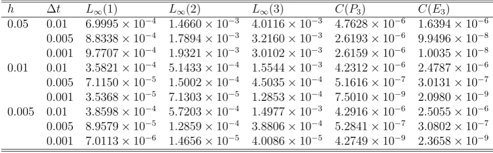
The discrete maximum norms computed at various times and the absolute relative changes computed at the simulation terminatig time t= 3 are tabulated in Table 2.
(a) Propagation of the single solitary wave (b) The maximum error distribution
Figure 1: The simulation of propagation of the single solitary wave and the maxi-mum error distribution att = 3 for h= 0.005 and ∆t= 0.001
with ∆t = 0.005 at t = 3. The choice of ∆t = 0.001 gives five decimal digit accurate solutions.
The initial values of the conservations laws are computed asE0 = 83
√
2(cosh21−1) sinh 1 =
4.431961243 andP0 = −83 √
2 cosh 1 =−5.819321497 analytically. These laws are expected to be constant during the simulation as time goes. The conservation of both laws during the numerical simulation is a good indicator of an efficient algorithm, Table 2.
The relative absolute change in the conservation law defining the momentum is less than 10−5whenh= 0.05. The choice ofhas 0.01 causes six and seven decimal digit relative absolute changes with respect to the ∆t choices as 0.01 and 0.005, respectively. The reduction of ∆t to 0.001 improves the relative absolute change to nine decimal digits.
When h is reduced to 0.005, the absolute relative changes of momentum are mea-sured as 4.2916×10⁻⁶, 5.2841×10⁻⁷ and 4.2749×10⁻⁹ for the choices of the ∆t
as 0.01, 0.005 and 0.001 respectively.
The absolute relative change of energy C(E3) is in six decimal digits at t = 3
Table 2: Discrete maximum norms and absolute relative changes of conservation laws at various times
h ∆t L∞(1) L∞(2) L∞(3) C(P3) C(E3)
0.05 0.01 6.9995×10⁻⁴ 1.4660×10⁻³ 4.0116×10⁻³ 4.7628×10⁻⁶ 1.6394×10⁻⁶
0.005 8.8338×10⁻⁴ 1.7894×10⁻³ 3.2160×10⁻³ 2.6193×10⁻⁶ 9.9496×10⁻⁸
0.001 9.7707×10⁻⁴ 1.9321×10⁻³ 3.0102×10⁻³ 2.6159×10⁻⁶ 1.0035×10⁻⁸ 0.01 0.01 3.5821×10⁻⁴ 5.1433×10⁻⁴ 1.5544×10⁻³ 4.2312×10⁻⁶ 2.4787×10⁻⁶
0.005 7.1150×10⁻⁵ 1.5002×10⁻⁴ 4.5035×10⁻⁴ 5.1616×10⁻⁷ 3.0131×10⁻⁷
0.001 3.5368×10⁻⁵ 7.1303×10⁻⁵ 1.2853×10⁻⁴ 7.5010×10⁻⁹ 2.0980×10⁻⁹ 0.005 0.01 3.8598×10⁻⁴ 5.7203×10⁻⁴ 1.4977×10⁻³ 4.2916×10⁻⁶ 2.5055×10⁻⁶
0.005 8.9579×10⁻⁵ 1.2859×10⁻⁴ 3.8806×10⁻⁴ 5.2841×10⁻⁷ 3.0802×10⁻⁷
0.001 7.0113×10⁻⁶ 1.4656×10⁻⁵ 4.0086×10⁻⁵ 4.2749×10⁻⁹ 2.3658×10⁻⁹
3.2
tanh-type Traveling Wave
In the second initial boundary value problem, we consider the caseε1 = 1,ε2 =−1
in the nonlinear Klein-Gordon equation. This choice of the parameter provides an analytical solution of the form
u(x, t) = tanh(p(x−ct)
2(1−c2)) (17)
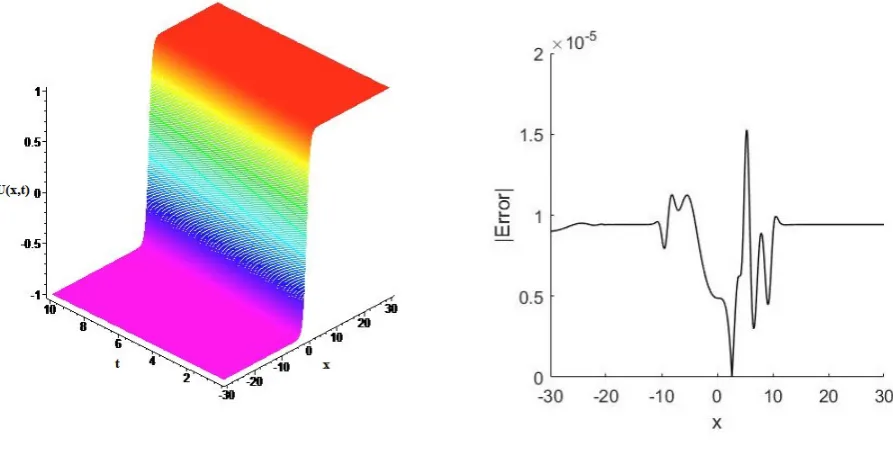
where c is the velocity of the traveling wave [34]. The existence of this real an-alytical solutions depends on the the condition −1 < c < 1. The wave travels along the x−axis to the right or to the left due to the sign of the velocity c. We choose the velocity c= 0.5 for the convenience. The initial data for the numerical solution is generated from the analytical solution (17) by substitutingt = 0 into it. The homogenous Neumann conditions at both end of the finite interval [−30,30] are used to complete the requirements of the iteration algorithm. The algorithm is run up to the terminating time t = 10 with various values of the discretization parametershand ∆t. The travel of the wave is simulated by the proposed algoritm successfully, Fig 2(a). The error takes its maximum values near points where the descent occurs as expected, Fig (2(b)).
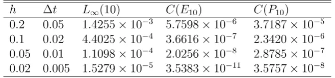
The discrete maximum norms and the absolute relative changes of the conser-vation laws are computed for various values of the discretization parameters are tabularised in Table 3. The accuracy of the proposed method at the time t = 10 is in three decimal digits when h and ∆t are chosen as 0.2 and 0.05, respectively. When the values of the discretization parameters are reduced to h = 0.1 and ∆t = 0.02, the maximum error is measured as 4.4025×10⁻⁴. Reducing the
(a) Traveling wave simulation (b) The maximum error distribution
Figure 2: Traveling wave simulation and the maximum error distribution att = 10
results but not in decimal digits. Finally, the choice of the parameters ash= 0.02 and ∆t= 0.005 gives a five decimal digit accuracy.
The initial values of the conservation laws describing the momentum and the energy are computed analytically as
E0 =−
1 9
405 e20
√
2√3+ 405 e40√2√3+ 12 e20√2√3√2√3 + ˜A
1 + 3 e20√2√3+ 3 e40√2√3+ e60√2√3 =−13.91133789
˜
A= 4√2√3−12 e40
√
2√3√
2√3−4 e60
√
2√3√
2√3 + 135 e60
√
2√3
+ 135
P0 =−2/9 √
2√3 =−0.5443310539
to h = 0.02 and ∆t = 0.005 improves the results to eleven decimal digits for the energy conservation and eight decimal digits for the momentum conservation law.
Table 3: Discrete maximum norms and absolute relative changes of conservation laws at various times
h ∆t L∞(10) C(E10) C(P10)
0.2 0.05 1.4255×10⁻³ 5.7598×10⁻⁶ 3.7187×10⁻⁵
0.1 0.02 4.4025×10⁻⁴ 3.6616×10⁻⁷ 2.3420×10⁻⁶ 0.05 0.01 1.1098×10⁻⁴ 2.0256×10⁻⁸ 2.8785×10⁻⁷
0.02 0.005 1.5279×10⁻⁵ 3.5383×10⁻¹¹ 3.5757×10⁻⁸
4
Conclusion
The collocation method based on trigonometric cubic B-spline functions combined with the Crank-Nicolson implicit method proposed for the solutions of two initial boundary value problems defined for the nonlinear Klein-Gordon equation. The aasumption v = ut reduced the order of the equation to one and generated a coupled system of partial differential equations. The system is integrated in time by using the Crank-Nicolson method and fully discretized by using the collocation method. Adapting the boundary conditions and arranging the initial state give a linear equation system for the iteration.
The validity of the proposed method is invesitgated by solving two initial boundary value problems. The propagation of a positive single solitary and travel of a wave are simulated successfully by the proposed method. The error between the numerical and analytical solutions are measured by using the discrete maximum norm. The conservation laws defining the energy and the momentum of the system are also computed by using the numerical results. The absolute relative changes of the convervation laws are also good indicators of the accuracy and validity of the proposed method.
References
[1] Whitham, GB: Linear and Nonlinear Waves, John Wiley & Sons, Newyork(1999).
[2] Debnath L: Nonlinear Partial Differential Equations for Scientists and Engi-neers, Birkhauser, Boston(2005).
[3] Detweiler, S: Klein-Gordon equation and rotating black holes. Phys. Rev. D, 22(10), 2323-2326 (1980).
[4] Galehouse, DC: Geometrical derivation of the Klein-Gordon equation. Int. J. Theor. Phys., 20(6), 457-479(1981).
[5] Weder, RA: Scattering theory for the Klein-Gordon equation. J. Func. Anal., 27(1), 100-117(1978).
[6] Lundberg, LE: Spectral and scattering theory for the Klein-Gordon equation. Commun. Math. Phys., 31(3), 243-257(1973).
[7] Ablowitz, MJ:Nonlinear Dispersive Waves, Cambridge University Press, Cam-bridge(2011).
[8] Sharma, AS, & Buti, B: Envelope solitons and holes for sine-Gordon and non-linear Klein-Gordon equations. J. Phys. A-Math. Gen., 9(11), 1823-1826(1976)..
[9] Dusuel, S, Michaux, P, & Remoissenet, M: From kinks to compactonlike kinks. Phys. Rev. E., 57(2), 2320-2326(1998).
[10] Kim, JJ, & Hong, WP: New solitary-wave solutions for the generalized reac-tion Duffing model and their dynamics. Z. Naturforsch. Pt. A, 59(11), 721-728 (2004).
[11] Burt, PB (1974). Solitary waves in nonlinear field theories. Physical Review Letters, 32(19), 1080.
[12] Huang, D. J., & Zhang, H. Q. (2005). The extended first kind elliptic sub-equation method and its application to the generalized reaction Duffing model. Physics Letters A, 344(2), 229-237.
[14] Chambers, L. G. (1966). Derivation of solutions of the Klein-Gordon equation from solutions of the wave equation. Proceedings of the Edinburgh Mathemat-ical Society (Series 2), 15(02), 125-129.
[15] Fleischer, W., & Soff, G. (1984). Bound state solutions of the Klein-Gordon equation for strong potentials. Zeitschrift f´’ur Naturforschung A, 39(8), 703-719.
[16] Burt, P. B., & Reid, J. L. (1976). Exact solution to a nonlinear Klein-Gordon equation. Journal of Mathematical Analysis and Applications, 55(1), 43-45.
[17] Kudryavtsev, A. E. (1975). Solitonlike solutions for a Higgs scalar field. Insti-tute of Theoretical and Experimental Physics.
[18] Ablowitz, M. J., Kruskal, M. D., & Ladik, J. F. (1979). Solitary wave colli-sions. SIAM Journal on Applied Mathematics, 36(3), 428-437.
[19] Campbell, D. K., & Peyrard, M. (1986). Solitary wave collisions revisited. Physica D: Nonlinear Phenomena, 18(1), 47-53.
[20] Strauss, W., & Vazquez, L. (1978). Numerical solution of a nonlinear Klein-Gordon equation. Journal of Computational Physics, 28(2), 271-278.
[21] Jim´enez, S., & V´azquez, L. (1990). Analysis of four numerical schemes for a nonlinear Klein-Gordon equation. Applied Mathematics and Computation, 35(1), 61-94.
[22] Dehghan, M., & Shokri, A. (2009). Numerical solution of the nonlinear Klein-Gordon equation using radial basis functions. Journal of Computational and Applied Mathematics, 230(2), 400-410.
[23] Sarboland, M., & Aminataei, A. (2015). Numerical solution of the nonlinear Klein-Gordon equation using multiquadric quasi-interpolation scheme. Univ J Appl Math, 3(3), 40-49.
[24] Cao, W. M., & Guo, B. Y. (1993). Fourier collocation method for solving nonlinear Klein-Gordon equation. Journal of Computational Physics, 108(2), 296-305.
[26] Zahra, W. K., Ouf, W. A., & El-Azab, M. S. (2016). A robust uniform B-spline collocation method for solving the generalized PHI-four equation. Ap-plications and Applied Mathematics, 11(1), 384-396.
[27] Dag, I., & Ersoy, O. (2016). The exponential cubic B-spline algorithm for Fisher equation. Chaos, Solitons & Fractals, 86, 101-106.
[28] Ersoy, O., & Dag, I. (2015). Numerical solutions of the reaction diffusion sys-tem by using exponential cubic B-spline collocation algorithms. Open Physics, 13(1).
[29] Korkmaz, A., & Dag, I. (2013). Cubic B-spline differential quadrature meth-ods and stability for Burgers’ equation. Engineering Computations, 30(3), 320-344.
[30] Korkmaz, A., & Dag, I. (2012). Cubic B-spline differential quadrature meth-ods for the advection-diffusion equation. International Journal of Numerical Methods for Heat & Fluid Flow, 22(8), 1021-1036.
[31] Abbas, M., Majid, A. A., Ismail, A. I. M., & Rashid, A. (2014, May). Nu-merical method using cubic trigonometric B-spline technique for nonclassical diffusion problems. In Abstract and applied analysis (Vol. 2014). Hindawi Publishing Corporation.
[32] Jhangeer, A., & Sharif, S. (2014). Conserved quantities for the non-linear Klein-Gordon equation. Afrika Matematika, 25(3), 833-840.
[33] Polyanin, A. D., & Zaitsev, V. F. (2004). Handbook of nonlinear partial dif-ferential equations. CRC press.
[34] Zaki, S.I., Gardner L.R.T., Gardner G.A., 1997, Numerical simulations of
Klein-Gordon solitary wave interactionsIl Nuovo Cimento, 112B, N.7.
c