Approximate Solution of
Forced Korteweg-de Vries Equation
Ong Chee Tiong, Mohd Nor Mohamad
&
*Samuel Shen Shanpu
Department of Mathematics,
Universiti Teknologi Malaysia,Skudai;
81310 Johor Bahru, Malaysia.
*Department of Mathematical Sciences,
University of Alberta,
Edmonton, Canada T6G 2G1.
Abstract Several findings on forced solitons generated by the forced Korteweg-de Vries equation (fKdV) are discussed in this paper. This equation has lost group symmetries due to the forcing term. The traditional group-theoretical approach can no longer generate analytic solution of solitons, because there are no infinitely many conservation laws. Approximate solution and numerical simulation seem to be the only way to solve fKdV equations. In this paper we show how approximate scheme can be used to solve the fKdV equation and generate uniform forced solitons. A detail derivation of the approximate solution was provided and various profiles of fKdV such as the depth of depression zone;
hd, amplitude; as, speed; s and the period;Ts of generation of forced uniform
solitons was given.
Keywords Forced soliton, uniform soliton, soliton collision and forced Korteweg de-Vries equation.
Abstrak Beberapa keputusan tentang penjanaan soliton paksaan oleh per-samaan paksaan Korteweg-de Vries (fKdV) telah dibincangkan dalam kertas kerja ini. Sistem persamaan seperti ini telah hilang sifat simetri kumpulannya akibat dari gangguan atau paksaan ke atasnya. Kaedah teori kumpulan tidak lagi mampu memberikan penyelesaian secara analitik kerana tidak wujud lagi ketakterhinggaan banyaknya hukum keabadian. Dengan itu kaedah penyelesa-ian secara penghampiran dan berangka sahaja yang mampu menyelesaikannya. Dalam kertas kerja ini kita akan tunjukkan bagaimana penyelesaian secara peng-hampiran mampu menyelesaikan persamaan fKdV dan seterusnya menjana soli-ton paksaan seragam. Penyelesaian hampir telah diterbitkan secara terperinci dan beberapa profil bagi fKdV seperti kedalaman zon tertekan; hd, amplitud;
as, laju;sdan tempoh;Tspenjanaan soliton paksaan seragam telah diberikan.
1
Introduction
In the last ten years, several researchers have conducted extensive studies on Korteweg-de Vries (KdV) equation and they were able to get free solitons generated, Shen (1993) [8]. With forcing terms added to the original KdV equation, it has lost group symmetries and the traditional group-theoretical approach can no longer generate analytical solution of solitons, because there is no infinitely many conservation laws. Approximate solution and numerical simulation seem to be the only way to solve fKdV equations, Shen(2002)[6].
When a fluid flow interacts with a topographic feature, and the fluid can support wave propagation, then there is the potential for waves to be generated upstream or downstream. In many cases when the topographic feature has a small amplitude, the situation can be successfully described by using a linearized theory and any nonlinear effects are determined as a small perturbation on the linear theory. However, when the flow is critical, that is, the system supports a long wave with zero group velocity in the reference frame of the topographic feature, then the linear theory failed and hence an intrinsically nonlinear theory need to be developed. It is now known that in many cases such a transcritical, weakly dispersive theory leads to a fKdV equation.
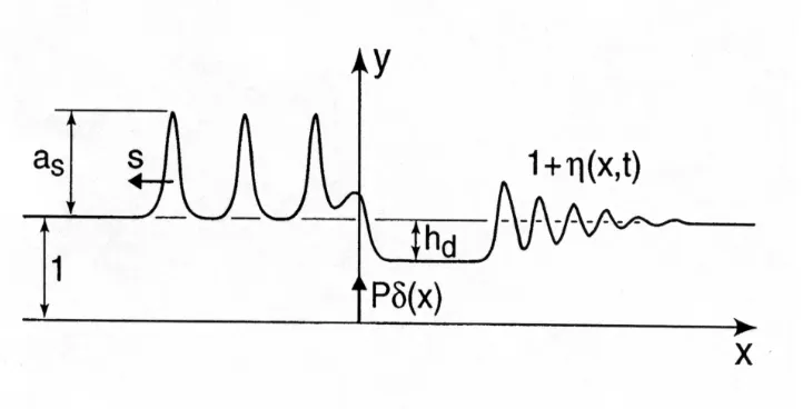
The first evidence of the existence of such solitons was provided by the celebrated discovery of the upstream radiated waves by a Caltech fluid mechanics group led by Wu T.Y. in 1982 [3]. This phenomenon is given in Figure (1). They claimed that these solitary waves are solitons.
Figure 1: An illustration of the schematic solution η(x, t) of fKdV for a fixed timet.
solution of solitons because there is no infinitely many conservation laws. Approximate solution and numerical simulation seem to be the only way to solve the forced nonlinear evolution equations in asymmetric systems.
In Section 2 we will derive the approximate solitary wave solution of fKdV and provide the profiles of fKdV solitons. Conclusion and discussion are given in Section 3.
2
Approximate Solution of fKdV
Since there is no analytical solution for fKdV equation and we would like to understand the behavior of forced solitons in fKdV, therefore an approximate scheme will be developed to solve the fKdV model given by equation (1).
ηt+ληx+ 2αηηx+βηxxx=
γ
2f
0
(x), −∞< x <∞. (1)
In this case, η(x, t) describes the free surface profile of the water flows over a bump, λ
measures the deviation of the bump speed from the shallow water velocity, γ is computed from the cross section area of the bump, whereas
f0(x) =δx(x)
is an isolated forcing function of Dirac-delta function,xis the spatial coordinate along the channel, t is time, α <0 and β < 0 are constants. The control parameters in this model are the bump size parameterγand the bump speed parameterλ. The initial condition for equation (1) isη(x,0) = 0 which is the water surface profile at rest. The solution consists of a forced soliton region generated upstream with amplitude;asand speeds, a depression
region with depthhd immediately on the lee side of the bump and a lee diminishing cnoidal
wave further downstream. The schematic solution of equation (1) is shown in Figure (1).
2.1
Derivation of Approximate Solution of fKdV
Thekth upstream soliton of the fKdV, Shen (1993),[8] may be expressed in the fol-lowing form
η(k)(x, t) =assech2
√ 3as
2 (x+st−δk)
, (2)
where δk is the specific phase shift for thekth soliton, sis the upstream advancing speed
of the solitons andas= 2(λ+s) is the amplitude of the soliton.
For each solitonη(k), with the first three conservation laws one has
m(sk)=
Z ∞
−∞
η(k)dx = 4has 3
i1 3
(mass )
Z ∞
−∞
(η(k))2dx= 8[2
3(λ+s)] 3
2 = 8
has
3
i3 2
(momentum )
Z ∞
−∞
[(η(k))3+1 3(η
(k)
x )
2
]dx= 32 3(λ+s)
5
2 = 4
√ 2 3 [as]
5
Based upon the mass balance postulate that the upstream soliton mass comes solely from the downstream depression when time is sufficiently large, one can derive approximate expressions of the depression depth hd, soliton amplitudeas, soliton propagation speeds,
and soliton generation periodTs in terms of the control parametersγ andλ.
In the stationary state withα=−34 andβ=−16, equation (1) can be reduced to;
ληx−
3 2η ηx−
1 6ηxxx=
γ
2δx(x). (3)
In this case, we know thatηt = 0 (stationary state),η(−∞) =hs and η(∞) =−hd.
By lettingη(x) =ξ(x) +hs, equation(3) becomes
λξx−
3
2(ξ+hs)ξx− 1 6ξxxx=
γ
2δx(x), (4)
and thus gives us
λ−3 2hs
ξx−
3 2ξξx−
1 6ξxxx=
γ
2δx(x), (5)
withξ(−∞) = 0 andξ(∞) =−(hs+hd).
Equation (5) is only solvable whenξ(x) is a smooth fall from the upstream zero solution to a downstream solitary wave tail. So λ−32hs<0 andξ(x) = 0 for allx in the domain
(−∞,0). Integrating equation (5) in the domain (0,∞) gives
λ−3 2hs
ξ−3 4ξ
2−1
6ξxx=
γ
2δ(x). (6)
In the case δ(x) = 0 ifx >0 and that reduce equation (6) is reduced to
λ−3 2hs
ξ−3 4ξ
2−1
6ξxx= 0, (7)
when x >0,ξ(0+) = 0;ξ
x(0+) =−3γandξ(∞) =−(hs+hd).
By integrating again equation (7) after multiplying by ξx the following expression is
obtained
2[λ−3 2hs]ξ
2−ξ3−1
3ξ
2
x+
1 3(9γ
2) = 0,
which can be further simplified into
1 3ξ
2
x= 2[λ−
3 2hs]ξ
2−ξ3+ 3γ2. (8)
Equation (8) is solvable only when the third order polynomial on the right hand side has a double roots. So,
2[λ−3 2hs]ξ
2−ξ3+ 3γ2= 0. (9)
4[λ−3
2hs]ξ−3ξ
2 = 0.
So, a root of this equation is
ξ = 4 3(λ−
3
2hs). (10)
Sinceξ(∞) =−(hs+hd),
hd = hs−
4
3λ. (11)
We know one of the roots of equation (9) is given byr0=43(λ−32hs) and if we substitute
it into equation (9) we obtain
hs =
2 3λ+ (
3γ2
4 ) 1
3, (12)
and
hd = (
3γ2
4 ) 1
3 −2
3λ. (13)
Equation (8) can now be written as
1 3ξ
2
x=ξ(s1−ξ)(ξ−s1+s2), (14)
where the roots are s1 = r1−r2 > 0 ; s2 = r1−r3 > 0 and r1, r2, r3 are roots of the equation. So thus equation (8) has a double roots and this give us r1 =r; r2 = r3 =r0
with r0= 43(λ−32hs). Therefores1 =r−r0 ands2 =r−r0=s1. So therefore equation
(14) becomes
1 3ξ
2
x = ξ
2(s1−ξ) (15)
ξx2 = 3ξ2(s1−ξ)
ξx =
√
3ξ p(s1−ξ) dξ
√
3ξp(s1−ξ) = dx
ξ = s1sech2 √
3s1
2 (x). (16)
Sinces1=hs=
2 3λ+ (
3γ2
4 ) 1
3 so we can replace it in equation (16) to obtain
ξ=
2
3λ+ ( 3γ2
4 ) 1 3 sech2 s 3[2 3λ+ (
3γ2
4 )
1
3]
4 (x). (17)
In order to know more profiles related to fKdV, we will integrate equation (1) from −∞to 0− with respect tox to obtain
Z 0−
−∞
ηtdx+λ
η 0− −∞ −3 4 η2 0− −∞ −1 6 ηxx 0− −∞ = γ
2δ(x)
0−
−∞
But the term
γ
2δ(x)
0−
−∞
is always zero in the region of (−∞,0−) and−1 6 ηxx 0− −∞ = 0
due to the “jump”. With this in mind equation (18) will become
Z 0−
−∞
η dx
t
+λη(0, t)−3 4η
2
(0, t) = 0. (19)
By letting
N =number of upstream solitons,
ms=mass of one soliton and
Ts=period of generating one soliton.
We can now define the rate of change of mass as
d dt
Z 0−
−∞
η1dx
!
=N ms
N Ts
=ms
Ts
,
so equation (19) will become
ms
Ts
=−λη(0, t) +3 4η
2(0, t). (20)
By integrating [equation (1) multiply byη(x, t)] from−∞to 0−with respect toxwill yield
Z 0−
−∞
ηηtdx + λ
Z 0−
−∞
ηηxdx−
3 2
Z 0−
−∞
η2ηxdx
− 1
6
Z 0−
−∞
ηηxxxdx=
γ
2
Z 0−
−∞
ηδx(x)dx.
This can be further simplified into
d dt
Z 0−
−∞
η2dx
!
= −λη2(0−, t) +η3(0−, t)
+ 1
3
η(0−, t)ηxx(0−, t)
−1 6
ηx2(0
−
, t)
. (21)
By denoting d
dt
Z 0−
−∞
η2dx
!
as the rate of change of momentum which is equal toN Mhs
N Ts
=
Mhs
Ts
; equation (21) becomes
Mhs
Ts
= −λη2(0−, t) +η3(0−, t)
+ 1
3
η(0−, t)ηxx(0−, t)
−1 6
ηx2(0−, t)
By intuitive observations, we will then make the following approximation lim T→∞ 1 T Z T 0
η(0−, t)dt=hs,
lim T→∞ 1 T Z T 0
η2(0−, t)dt=h2s,
lim T→∞ 1 T Z T 0
η3(0−, t)dt=h3s,
lim T→∞ 1 T Z T 0
η(0−, t)η1xx(0−, t)dt= 0,
lim T→∞ 1 T Z T 0
η12x(0−, t)dt= 0.
By using the above approximation we will simplify equation (20) and obtained
ms
Ts
=−λ hs+
3 4h
2
s. (23)
By using the same approximation we will simplify equation (22) and obtained
Mhs
Ts
=−λ h2s+h3s. (24)
By dividing equation (24) by equation (23) we get the important relationship
Mhs
ms
= −λ h
2
s+h3s
−λ hs+34h2s
= −λ hs+h
2
s
−λ+34hs
. (25)
But we know that the mass one soliton is given by
ms=
Z ∞
−∞
η(k)dx= 4has 3
i1 3
,
and the momentum of one soliton is given by
Mhs=
Z ∞
−∞
(η(k))2dx= 8[2
3(λ+s)] 3
2 = 8
has
3 i3 2 , therefore Mhs ms = 8[ as 3] 3 2
4[as
3]
1 3
=2
3as. (26)
By equating equation (26) to equation (25) we get the amplitude of forced solitons as given by
2 3as =
−λ hs+h2s
−λ+34hs
as =
3 2
h
s(−λ+hs)
−λ+3 4hs
as = 2
(h
d+43λ)(hd+13λ)
hd
Again we will integrate equation (1) from−∞toxD with respect tox, that will yield
Z xD
−∞
ηtdx + λ
Z xD
−∞
ηxdx−
3 2
Z xD
−∞
ηηxdx
− 1
6
Z xD
−∞
ηxxxdx=
γ
2
Z xD
−∞
δx(x)dx. (28)
Equation (28) then becomes
Z xD
−∞
ηtdx+λ
η xD −∞ −3 4 η2 xD −∞ −1 6 ηxx xD −∞ = γ 2
δ(x)
xD
−∞
. (29)
By substituting the approximation that we have made earlier; equation (29) will yield
ms
Ts
+λ hs−
3 4h
2
s = 0
ms
Ts
= 3
4h
2
s−λ hs
Ts =
ms
3
4h2s−λ hs
Ts =
4[as
3] 1 2 3 4h 2
s−λ hs
Ts =
16 3
2(h
d+13λ)
3h3d(hd+43λ)
1 2
. (30)
2.2
Profile of fKdV Solitons
From the above derivations, which is based upon the mass balance postulate that the upstream soliton mass comes solely from the downstream depression zone when time is sufficiently large, one can derive approximate expressions of the depression depthhd, soliton
amplitudeas, soliton propagation speeds, and soliton generation periodTs, in terms of the
control parametersγ andλ, Shen(2002) [6] given as
hd = {
3 4γ
2}1
3−2
3λ, (31)
as =
2(hd+43λ)(hd+13λ)
hd
, (32)
s = as
2 −λ, (33)
Ts =
16 3
2(h
d+13λ)
3h3
d(hd+
4 3λ)
1 2
. (34)
2.3
Dirac-delta Forcing in fKdV Equation.
The forcing function in equation (1) given by γ2f0(x) which may due to the bottom
topography of the fluid domain (such as a bump on the bottom of a two dimensional channel), or due to an external pressure on the free surface (such as the wind stress on the surface of an ocean). By taking f0(x) = δ
x(x) which is a Dirac-delta forcing as in Shen
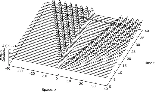
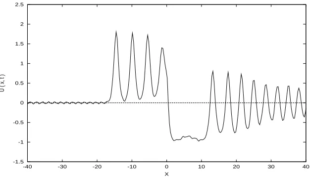
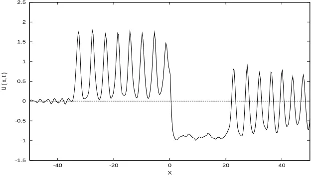
(1996), [9], γ = 1 and if we keep λ= 0 so as to remain in the transcritical region we are able to observe the generations of forced uniform solitons as given by Figure 2 which shows the 3D plot of the forced uniform solitons propagations. At a specific time t = 10,t = 20,
t = 30 and t = 40 we observe that the solution to equation (1) was given by Figure 3, Figure 4, Figure 5 and Figure 6 respectively. The approximate solution of the nonlinear partial differential equation (1) with the depth of depression zone hd, amplitudeas, speed
s and generation period Ts of the matured uniform forced solitons can be calculated from
the above approximate expression. For λ= 0 and γ= 1.0 the profiles are:
hd= 0.9086, as= 1.8172, s= 0.9086, and Ts= 5.0280.
-40 -30
-20 -10
0 10
20 30
40
Space, x 0
5 10
15 20
25 30
35 40
Time,t -1
-0.50.50 1 1.52 2.53
U ( x , t )
Figure 2: Uniform Solitons Generated by Dirac delta Forcing (3D Plot).
In Figure 3, when t= 10<2Tswe can only observe one matured soliton and another
-1.5 -1 -0.5 0 0.5 1 1.5 2 2.5
-40 -30 -20 -10 0 10 20 30 40
U ( x, t )
X
Figure 3: Generations of Forced Solitons att= 10 (2D Plot).
-1.5 -1 -0.5 0 0.5 1 1.5 2 2.5
-40 -30 -20 -10 0 10 20 30 40
U ( x, t )
X
Figure 4: Generations of Forced Solitons att= 20 (2D Plot).
In Figure 5, whent= 30<6Tswe can only observe only 5 matured soliton and another
-1.5 -1 -0.5 0 0.5 1 1.5 2 2.5
-40 -30 -20 -10 0 10 20 30 40
U ( x, t )
X
Figure 5: Generations of Forced Solitons att= 30 (2D Plot).
In Figure 6, whent= 40<8Tswe can only observe only 7 matured soliton and another
soliton emerging and will be matured at t= 40.224.
-1.5 -1 -0.5 0 0.5 1 1.5 2 2.5
-40 -20 0 20 40
U ( x, t )
X
Figure 6: Generations of Forced Solitons att= 40 (2D Plot).
3
Conclusion and Discussion
and γ we do generates forced uniform solitons and we know the profiles of each forced uniform solitons generated. With this new findings, we have another resource to confirm our research results with other schemes namely the numerical simulation or even with the analytical solution of fKdV if ever found.
References
[1] Camassa, R. and Wu, T.Y., “Stability of Forced Steady Solitary Waves”, Phil. Trans. Royal Society of London A 337,1991, pg 429-466.
[2] Lax, P.D,“Integrals of Nonlinear Equations of Evolution and Solitary Waves”, Comm. Pure Appl. Math, Vol 21,1968, Pg 467-490.
[3] Lee, S.J., Yates, G.T. and Wu, T.Y,“Experiments and analyses of upstream advancing solitary waves generated by moving disturbances”, J. Fluid Mech 199,1989, pg 569-593.
[4] Nouri, F.Z and Sloan, D.M., “A comparison of Fourier Pseudospectral Methods For The Solution of the Korteweg de Vries Equation”, Journal of Comp. Phys. 83,1989, pg 324.
[5] Ong, C.T.,“Various Aspects of Solitons Interactions”, M.Sci. Thesis (Applied Mathe-matics), Universiti Teknologi Malaysia, 1993.
[6] Shen, S.S.P., Shen, B.,Ong, C.T.,and Xu, Z. T.,“Collision of Uniform Soliton Trains in Asymmetric Systems”, DCDIS Series B: Applications & Algorithms, 9, 2002, pg 131-138.
[7] Redekopp, L.G. and You, Z.,“Passage through resonance for forced Korteweg-de Vries equation”, Phys. Rev. Lett., 74,1995, pg 5158-5161.
[8] Shen, S.S.P.,“A Course on Nonlinear Waves”, Kluwer,1993.
[9] Shen, S.S.P., Manohar, R.P. and Gong, L., “Stability of the lower cusped solitary waves”, Phys. Fluids, A 7,1995, pg 2507-2509.
[10] Shen, S.S.P., “Energy Distribution For Waves in Transcritical Flows Over a Bump”, Wave Motion 23,1996, pg 39-48.