1 Faculty of Geo-Information Science & Earth Observation (ITC), University of Twente, Enschede 7514 AE, 6
The Netherlands; E-mails: [email protected]; [email protected]; [email protected]; 7
* Correspondence: [email protected]; Tel.: +31-534-874-301 9
10 11
Abstract: Object-Based Image Analysis (OBIA) has been successfully used to map slums. In general, 12
the occurrence of uncertainties in producing geographic data is inevitable. However, most studies 13
concentrated solely on assessing the classification accuracy and neglecting the inherent 14
uncertainties. Our research analyses the impact of uncertainties in measuring the accuracy of OBIA-15
based slum detection. We selected Jakarta as our case study area, because of a national policy of 16
slum eradication, which is causing rapid changes in slum areas. Our research comprises of four 17
parts: slum conceptualization, ruleset development, implementation, and accuracy and uncertainty 18
measurements. Existential and extensional uncertainty arise when producing reference data. The 19
comparison of a manual expert delineations of slums with OBIA slum classification results into four 20
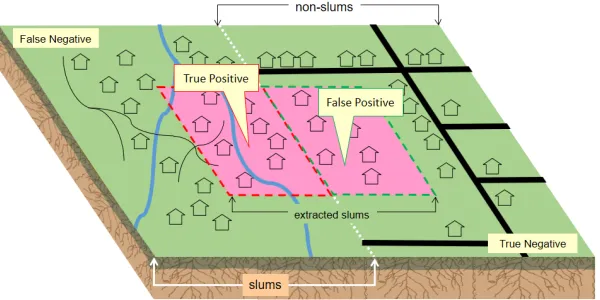
combinations: True Positive, False Positive, True Negative and False Negative. However, the higher 21
the True Positive (which lead to a better accuracy), the lower the certainty of the results. This 22
demonstrates the impact of extensional uncertainties. Our study also demonstrates the role of non-23
observable indicators (i.e., land tenure), to assist slum detection, particularly in areas where 24
uncertainties exist. In conclusion, uncertainties are increasing when aiming to achieve a higher 25
classification accuracy by matching manual delineation and OBIA classification. 26
Keywords: Accuracy; Uncertainties; Object-Based; Slums; Jakarta 27
28
1. Introduction 29
The most recent global target in slum reduction stated in the Sustainable Development Goals 30
(SDG) is to ensure access to adequate, safe and affordable housing and essential services for all people 31
by 2030 [1]. Although the target has been stipulated, the number of slum dwellers is growing. In 2012, 32
the number of dwellers living in urban slums was 863 million, which increased from 776 to 827 and 33
881 million in 2000, 2010 and 2015 respectively [2,3]. Highly dynamic changes in cities and slums 34
require techniques that can provide rapid and reliable information for policy formulations related to 35
slums. However, information regarding the growth and expansion of slums is sparsely available [4]. 36
Survey-based data collection methods have limitations due to long temporal gaps and the degree of 37
aggregation [5]. Thus, data might be obsolete when being used [6]. Meanwhile, although satellite 38
imagery gives the opportunity to provide almost real-time information [6], slums and non-slums 39
often share similar surface materials [7], and slum morphologies differ within and across cities [8], 40
which makes their identification somehow difficult. 41
Among various approaches that were developed, Object-Based Image Analysis (OBIA) has an 42
excellent potential to extract slums using spectral as well as contextual information through a 43
hierarchical procedure [9]. However, often the classification process is context and data dependent 44
[6] and not flexible to be applied to a different place (city), different images (sensor and different 45
date). The development of the Generic Slum Ontology (GSO) aimed to bridge this gap [6,9], by 46
providing a complete characterization of slums using morphological indicators [7] at three spatial 47
levels, i.e., environs, settlement and object [10]. This characterization was developed by adopting the 48
durable housing indicator from UN-Habitat [5]. 49
Although the GSO assists in slum detection, it provides a generic concept of slums [11], while 50
slums can show considerable diversity within a city and even within a settlement [7,12]. For instance, 51
same characteristics (e.g., density), often differ locally and depend on developmental stages of 52
settlements [5]. Therefore, settlements having similar densities might be considered as slums in one 53
place but as non-slums in another place [13]. This illustrates challenges faced when aiming at a 54
transferable slum mapping approach based on a set of generic indicators. 55
The above-mentioned variability (e.g., spatial, temporal, sensors) requires a local adaptation of 56
the GSO. In the OBIA context, adaptations of such a ruleset for different images are inevitable 57
[7,14,15]. Nonetheless, it is crucial to promote transparency of the adaptations to ensure objectivity 58
[14], in measuring transferability of the ruleset [16]. Here, transferability is defined as the degree of 59
adaptations of a ruleset to produce comparable results from different imaging conditions [7]. 60
Previous studies on OBIA-based slum detection focus either on comparability of the results [7,15] or 61
on the degree of adaptations [17,18] and both approaches use accuracy as a benchmark. 62
Measuring transferability by only considering the accuracy indicators as a benchmark has some 63
shortcomings. First, the occurrence of uncertainties in producing geographic data is inevitable [19], 64
and the level of uncertainties will propagate through the whole process chain [20]. Second, in OBIA, 65
manual image interpretation is commonly used as reference data [21], often producing ambiguous 66
results as some interpreters delineate more detailed objects and the others may generalise objects [22]. 67
Third, it is hard to define the exact transition between slums and non-slums [23]. Fourth, the 68
differences in experience and the way to conceptualise slums among interpreters may lead to 69
different delineations of reference data [23]. Hence, reflecting on the uncertainties mentioned above, 70
it is crucial to consider these in the accuracy assessment for OBIA classifications [22]. 71
In this paper, we analyse the impact of uncertainties in producing reference data for the accuracy 72
assessment of OBIA-based slum detection. We organised our study into four sections. First, we 73
describe our case study. Second, we discuss materials and methods, which includes the development 74
of OBIA rulesets, accuracy and uncertainties measurements. Third, we discuss the results and fourth, 75
we present the conclusions of our research. 76
2. Case Study 77
Jakarta, the capital city of Indonesia, has grown enormously since a half-century ago, and its 78
metropolitan area is home to more than 30 million inhabitants [24]. The magnitude of economic 79
activities and the presence of numerous societal infrastructures attract rural people to Jakarta. 80
However, the lack of capacities by the local government in providing affordable housing has forced 81
low-income households to settle in substandard housing areas [25]. Thus, Jakarta is facing challenges 82
in terms of managing its rapid demographic and economic growth, which also affects the growth of 83
slums [26]. Approximately, 60% of Jakarta’s population, predominately from a low-income 84
household, are living in informal settlements called kampungs. 85
At the national level, the Government of Indonesia has set the 100-0-100 policy (100% access to 86
clean water, 0% slums, 100% access to sanitation) as part of the Medium Term National Development 87
Program (RPJM) [27]. The national government committed 9.5 billion US Dollars from the national 88
budget until 2019 for this purpose [28]. Hence, to monitor the slum dynamics is key to determine the 89
success of implementing this policy [29]. For this purpose, reliable and updated information on slums 90
is required. 91
In general, to define slum boundaries in Jakarta is not straightforward. Informal developments 92
in Jakarta started a half-century ago when Jakarta experienced rapid urbanisation [30], at that time 93
the planning institutions were not established [31]. Locally, these informal settlements are called 94
according to the housing quality and mentioned that slum building can be characterized by inadequate living space [35]. Meanwhile, the Ministry of Public Works developed indicators 106
according to the quality of settlements, where slums can be characterized by its under-served facilities 107
[36]. Internationally, the most commonly employed definition of a slum is based on the durable 108
housing indicators, where a slum is an area that is characterised by lack of access to safe water and 109
sanitation, low building quality, overcrowded and lacks tenure security [37]. 110
For the purpose of this study, we selected a subset around Tebet district (sized 29 square 111
kilometres) in Jakarta (Figure 1) due to three reasons. First, Tebet district comprises of various land 112
uses namely high-income residential areas, shopping arcade, the centre of the transportation hub, 113
and slums. Second, the Ciliwung river that is locally associated with slums flows through this district. 114
Third, the district houses various types of slums (e.g., slums that are located on the riverbank, near 115
the railroad, near the CBD). 116
(a) (b)
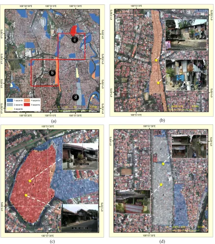
Figure 1. Map of the study area in Jakarta Province (Indonesia) (a), surrounded by Banten Province 117
and West Java Province (the metropolitan area includes some parts of these provinces), area boundary 118
source: Openstreet Map (2015). (b) Selected subset located in Tebet district, Jakarta. Image Source: 119
Google Earth (2015). 120
3. Materials and Methods 121
Our research methods comprise of four main parts: (i) slums conceptualisation, (ii) OBIA ruleset 122
development, (iii) ruleset implementation, (iv) accuracy and uncertainty measurement. Our 123
125
Figure 2. Research methodology comprising of four main parts and its following activities. 126
In the first part, we related the definitions of slums by the local experts with image-based 127
information by using several observable visual elements, e.g., tone, shape, size, texture and 128
association [6,10]. We selected five local experts from different backgrounds, i.e., government, 129
consultants and NGO. As mentioned in [23], the selected experts needed to have a professional 130
knowledge on slums. Therefore, we selected experts that have been involved in programs related to 131
slums in Jakarta. From the government, we have interviewed two experts, one from the National 132
Government (Ministry of Public Works), and one from the Local Government (Department of Spatial 133
Planning, Jakarta). In addition, we interviewed two experts from consultancies that were involved in 134
formulating the national policy of slums in Indonesia. Lastly, we interviewed one representative from 135
an NGO, who participated in monitoring settlement targets for the Millennium Development Goals 136
(MDG). Besides expert interviews, field observations were conducted in the areas experts delineated 137
as slums. The characteristics of slums obtained during the interviews were used for developing the 138
ruleset for the OBIA-based slum detection. 139
In the second part, we developed the OBIA-based ruleset for slum detection according to the 140
definitions mentioned in the first step. In general, OBIA aiming to relate geographic features with 141
image objects can be divided into two main parts, namely segmentation and classification [38]. In 142
general, segmentation delineates regions (segments) of an image which share common attributes [39]. 143
The result is a relatively homogeneous and significant grouping of pixels [40]. Meanwhile, the 144
classification process assigns each segment to a particular class according to predefined 145
characteristics, e.g., tone, shape, size, texture and association. For segmentation, we used multi-146
resolution segmentation (MRS) since this algorithm has been widely used in OBIA-based slum 147
detection studies (e.g. [5,12]). However, the implementation of MRS is depended on the Scale 148
Parameter (SP) [41], controlling the heterogeneity of image objects [42]. The SP value is often selected 149
in a trial-and-error process [43]. Therefore, we employed the Estimation Scale Parameter (ESP) tool 150
[41] to determine the most appropriate SP. 151
In the third part, we implemented the ruleset in our study area. We selected Pleiades imagery 152
granted from the European Space Agency (ESA) with standard-ortho bundles for the year of 2015, 153
with a spatial resolution of 0.5-meter for R-G-B-NIR bands. We managed to obtain an image with a 154
cloud cover of less than 10%. We purposively selected two small test areas (sized 1 square kilometres), 155
without any cloud cover. For the first test area, we selected an area with a relatively similar agreement 156
of slum boundaries among experts, while in the second area, experts considerably disagreed about 157
slum boundaries. 158
Lastly, in the fourth part, we measured the accuracy of the classification result. Manual 159
delineation of slum boundaries (on top of the image) by local experts were used to produce the 160
reference data, as demonstrated in [22,23]. Thus, we compared the extracted slums from the OBIA 161
ruleset, with the reference data from the local experts. This comparison, obtained four possible results 162
164
Figure 3. Four possible results from combining classification result with the reference data produced 165
by the experts. 166
We used three indicators for measuring accuracy, i.e., precision, recall and accuracy. Precision 167
or confidence describe the proportion of predictive-positive cases, which show a correct match with 168
the reference data [44]. It can be measured by comparing TP with TP and FP (1). Meanwhile, recall or 169
sensitivity indicates the proportion of real positive cases that were correctly predicted, and it 170
indicates the degree of the confidence of our classifiers. It can be measured by comparing the number 171
of TP, with TP and FN (2). Lastly, accuracy indicates the total correct positive and negative cases (i.e., 172
TP and TN) to the total number of possible cases (i.e., TP, FP, FN, TN) (3) [44]. Therefore, precision, 173
recall and accuracy were calculated as: 174
=
+ (1)
=
+ (2)
= +
+ + + (3)
Regarding uncertainties, as pointed out in [23], the difficulties to draw exact boundaries where 175
slums change into non-slums and vice versa leading to uncertainty, i.e., existential and extensional 176
uncertainty [45]. First, existential uncertainty indicates the degree of confidence whether a slum exists 177
in reality [23,45], and it may depend on experts’ experience or conceptual difference upon image 178
interpretations [23]. Second, extensional uncertainty indicates the area delineated as a slum with 179
limited certainty [23]. 180
Furthermore, uncertainties also arose from different slum conceptualizations by local experts. 181
While [23] aimed to study the deviations of slum boundaries observed from VHR images, our 182
research emphasises the impact of various degrees of slum boundaries’ agreements on the values of 183
the accuracy assessment. To do so, we compared the classification result (OBIA slum map for each 184
test area) obtained in the third part with the reference data showing various agreement levels. For 185
instance, first, we compared the classification result with an area where the reference data showed 186
the highest agreement (all five experts agreed that an area is a slum). Next, we measured the accuracy 187
according to the indicators mentioned in (1) to (3). We repeated this procedure for each subset and 188
every degree of agreement (ranging from 1-5 experts). This comparison allowed us to examine the 189
impact of different agreements in the reference data on accuracy levels for mapping slums in Jakarta. 190
3. Results 191
The result of the expert interviews shows the local diversity of slum characteristics (Table 1). The 193
expert from the national institutions (i.e., Ministry of Public Works) defined slums according to the 194
building size, which in general, is smaller in size compared to non-slum buildings. In addition, slums 195
are located commonly on the riverbank or near railroads, with irregular building orientations. The 196
expert from the local government mentioned similar characteristics regarding the location on the 197
riverbank and near railroads. With regards to the difficulties to distinguish slum and non-slum 198
kampungs, the tenure status was often mentioned as a characteristic that could be used for 199
distinguishing. Experts (NGO and two consultants) also came up with the slum characteristic of small 200
building sizes. In addition, they also mentioned that slums have irregular building orientations, poor 201
roof materials and are located on the riverbank and near railroads. The last expert (the second 202
consultant), however, only mentioned building size and irregular building orientation as slums 203
characteristics. 204
Table 1. Different characteristics and definitions of slums among local experts. (1) is from the central 205
government; (2) is from the local government; (3) is from Non-Government Organization (NGO), 206
and (4) and (5) are housing policies consultants. 207
Characteristics Local Expert
(1) (2) (3) (4) (5)
1 Located on/close the river bank/railroad √ √ √ √
2 Small building size √ √ √ √
3 Irregular building orientation √ √ √ √
4 Poor roof material √ √ √
5 Built on illegal land √
According to the visual image interpretations, local experts have different agreements on slum 208
locations in our study area. In Error! Reference source not found.4 a, we show the different 209
agreements of slum extents (delineated by experts), where the red area and blue areas indicate the 210
highest and lowest agreement respectively. To give a better understanding regarding slum 211
characteristics on the ground, we conducted field observations. For the first sample (Error! Reference 212
source not found.4 b), we selected an area along the Tebet Timur Street, which was digitized by 4 of 213
our experts. From field observations, this area is characterised by its proximity to the river and has 214
irregular building orientations. We also found that buildings in this area are made up of poor 215
materials (e.g., cardboard, plastics, corrugated iron, woven bamboo). In addition, we noticed 216
different types of roof materials (i.e., ranging from tiles to corrugated irons). For the second example, 217
we selected an area in Manggarai I street (Error! Reference source not found.4 c), which shows 218
(a) (b)
(c) (d)
Figure 4. Slums extracted from manual delineation by different experts. Figure (a) shows the different 220
agreements of slum extents, where the red colour indicates areas with the highest agreement and the 221
blue colour indicate the lowest. Figure (b) shows the ground conditions of slums were four experts 222
agreed. Figure (c) shows the ground conditions of slums, which were indicated as a slum by all 223
experts. Figure (d) shows the ground conditions of a slum that was selected by one and two experts. 224
The red boxes in Figure (a) indicate our test areas. 225
3.2. OBIA Ruleset Development 226
When developing the OBIA ruleset, we translated the characteristics of slums obtained from the 227
local experts, into characteristics that can be recognised by a computer. The association may include 228
tone, shape, size, texture and associations. Table 2 shows the five characteristics of slums that are 229
used to develop ruleset. 230
Table 2. Translation of the real world characteristics into image domain characteristics in the context 231
Real world domain Image domain 1 Located on the riverbank/near railroad Association: Distance to River/Railroad 2 Small building size Size: Small
3 Irregular building orientation Shape: compactness
4 Poor Roof material Tone: Asbestos, corrugated iron 5 Built in the illegal land Ancillary data: Land Use Plan
For the first characteristic, slums are commonly located on the riverbank or near the railroad. 233
Thus we employed a vector layer of rivers and railroad (Openstreet Map data) using proximity as a 234
rule. For the second and third characteristics, we associate the size and shape of the building with the 235
shape and size of the segment. Meanwhile, for the fourth characteristic, we associate the roof material 236
of slum buildings with the tone/colour of the segment. The last characteristic is most interesting. 237
Unlike the four previous characteristics, the last one is not directly observable from an image. 238
Therefore, we used a proxy indicator to determine the tenure status. According to the interview with 239
the expert from the Jakarta province, Jakarta is implementing a strict zoning regulation, which means 240
it is illegal to construct within protective zones. Thus, we decided to use the zoning map to delineate 241
the protected zones, where any construction is illegal and has no legal tenure status. 242
The idea of using a non-observable indicator has induced us to develop two scenarios when 243
implementing our ruleset. First, we run our ruleset with four indicators (only observable; indicator 244
number 1 to 4 in Table 2). Second, we include the non-observable indicator (number 5 in Table 2). We 245
applied both scenarios for the two test area. 246
After we associate each slum characteristic with its consecutive image domain, we develop our 247
ruleset in Trimble’s eCognition software. Our ruleset can be divided into two steps (Figure 5). First, 248
background removal and second, slum detection. In the background removal step, we implement 249
MRS with a low SP (SP=1) to extract background classes, i.e., vegetation, railroads, roads, and the 250
rivers. Next, we apply a coarse segmentation for the remaining unclassified segments, here we 251
implement our ruleset for slum detection. 252
253
Figure 5. OBIA ruleset flowchart, which starts with background removal, followed by slum detection. 254
In the first step, we find that among various possible associations (i.e., tone, shape, size, texture 255
and associations), which can be used for classification, the Normalized Difference Vegetation Index 256
(NDVI: proportion between near-infrared and red band) shows its ability to detect the vegetation 257
well. Each object that has an average value of NDVI greater than zero is classified as vegetation. 258
However, if we choose a coarse segmentation, vegetation is under-segmented (Figure 6). Hence, we 259
are intentionally over-segmenting, because we aim to obtain the shape and size of the vegetation class 260
(a) (b) (c)
Figure 6. Impact of segmentation scale on vegetation classification. Figure (a) shows segments with a 262
NDVI of greater than zero obtained from fine segmentation and (b) from coarse segmentation, and 263
(c) image before segmentation process. 264
For the remaining background classes (i.e., road, railroad, river), we classify the segments using 265
vector data. For this purpose, we also implemented a fine segmentation for these classes. After we 266
classified all background classes, the remaining class (i.e., unclassified) has a certain probability to be 267
classified as a slum. Here, we implement the second step. 268
In this second step, we re-segment the unclassified class, aiming at coarser segments. The ESP 269
can produce three levels of segmentation, which can be associated with three level of slums object as 270
mentioned in [5]. Since slum buildings are characterised by its small size (Table 2), it is difficult to 271
extract every single building as an object. Therefore, we use the second level of SP obtained from ESP, 272
which is 95. 273
After conducting the segmentation process, we implement our concept of slums to develop the 274
ruleset for classifying each test area. The threshold values were obtained through a trial and error 275
process, and we assigned these values into the class description in E-cognition software (Table 3). 276
Table 3. Threshold value for each rule 277
Rule Threshold value
Association: Distance to River/Railroad 1. Border to river >0 pixels
2. Border to railroad 0 > pixels
Shape: compactness 1. Compactness ≤ 5
2. GLCM Dissimilarity ≥ 0.0005
Tone: tile – corrugated iron, asbestos Mean red/green 1 ≤ tone ≤ 1.075
Ancillary data: Land Use Plan (second scenario) Mean Layer Tenure >0.25 278
For the first rule, we use the border to the river and railroad, and assign each object that has 279
more than zero pixels touching the border of river/railroad as a slum. Regarding shape, we 280
implement two rules, compactness and grey level co-occurrence matrix (GLCM) dissimilarity. 281
Compactness indicates the variations among pixels under one object. The lower the compactness, the 282
higher the variation of pixel values. Regarding GLCM dissimilarity, the higher the value, the pixel 283
values show lesser similarity within one segment [46]. For the tone, since the roof materials of slum 284
houses in our study area are predominated by tiles or corrugated iron, we find that average of 285
red/green shows a linear relationship with the roof colour. Here, we use the band arithmetic approach 286
in E-cognition by calculating the proportion of red and green band in each segment. The last rule is 287
only applicable for the second scenario. To develop this rule, we first converted the zoning map of 288
the study area from vector to raster. Then, we reclassified the value of each land use class into two 289
the ‘tenure value’ of each segment and identify the threshold for slums. The more the segmented 291
image overlapped with the ‘tenure segment’, the higher the chance that the segment is a slum. 292
We use “OR” function for association in our ruleset, which means that a slum may be located 293
near the river, or near the railroad, or in the proximity of both of them. Meanwhile, for the rest of the 294
indicators, we use “AND” function, which means that the object must meet all threshold value to be 295
classified as slums. 296
3.3. Ruleset Implementation 297
We implement our ruleset in the first test area (clear boundaries between slum and non-slum), 298
and the second area (unclear boundaries). Also, we implement our ruleset for two scenarios, first with 299
using tenure status as an additional proxy, and second without tenure status. Hence, the four pairs of 300
results are shown in Figure 7. 301
(a) (b)
(c) (d)
Figure 7. Mapped slums in the first test area (a,b). Figure (a) indicates slums without the tenure 302
indicator (only consider explicit indicators) (b) indicates slum employing the tenure indicator. 303
Meanwhile, figure (c) and (d) indicates slums in the second area, by including and excluding the 304
3.4. Accuracy and Uncertainty Measurements 315
Each classification results shown in Figure 7, we compared with the degree of agreements by 316
experts, which ranges from five (highest agreement) to only one agreement (only selected by one 317
expert (reference data). This results in twenty possible values for each accuracy indicator mentioned 318
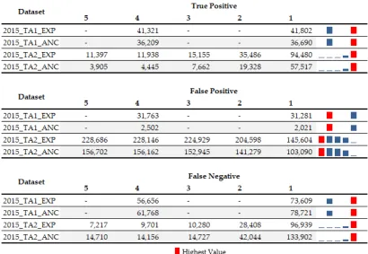
in Equation (1) to (3). Figure 8, shows the size of true positive (TP), false positive (FP) and false 319
negative (FN), measured in square meters. 320
321
Figure 8. The size (in m2) of true positive, false positive and false negative obtained by comparing 322
classification results with the level of agreement. 2015_TA1_EXP indicates the year of the image, TA1 323
gives the location of the first test area (TA). EXP indicates that we only used explicit/observable 324
indicators, while on ANC means that we include an ancillary (not observable in images) indicator. 325
The number of TP indicates the size of the area that is detected as slums by the OBIA 326
classification as well as in the reference data. We find differences in the amount of TP between TA1 327
and TA2, also between EXP and ANC. Apparently, the difference between EXP and ANC in TA1 is 328
lower than in TA2. Both areas and scenarios show similarities related to the number of agreements. 329
As we reduce the required degree of agreements for the reference data (from 4 to 1 in TA1, and from 330
5 to 1 in TA2), the size of TP is increasing. However, we only find two degrees of agreement in TA1 331
(i.e., one and four experts). Meanwhile, we find various levels of agreements in TA2, which indicates 332
FP indicates the size of the area, which is detected as slums from by the OBIA classification but 334
not delineate as slums by the experts. Interestingly, the difference of FP between EXP and ANC in 335
TA1 is substantially greater than in TA2. In TA1, the size of FP in EXP is thirteenth times higher than 336
ANC. Meanwhile, the difference of FP in TA2 for EXP is only one-and-half time greater than ANC. 337
TA1 and TA2 show similarities related to the degree of agreements. As we reduce the degree, we get 338
a decreasing number of FP. 339
Lastly, the FN indicates the size of the area that is detected as a slum by the experts but not 340
detected as a slum by the OBIA classification. We notice a similar pattern of FN between EXP and 341
ANC in TA1 and TA2. As we decrease the number of required agreements, we have an increasing 342
number of FN. However, the increasing of FN in TA1 (for EXP and ANC) is more gradual than in 343
TA2. In TA2, we find a significant increase of FN when we reduce the agreement from 2 to 1. This 344
points to very diverse perceptions by experts on slum boundaries in TA2. Therefore, it results in a 345
substantial size of slum patches with only one agreement, Figure 4 (a) in the red box labelled c. 346
Using the value of TP, FP and FN, we calculate precision, recall and accuracy using Equation (1) 347
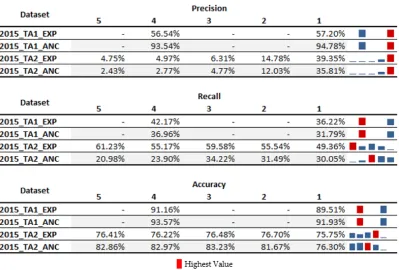
to (3), shown in Figure 9. 348
349
Figure 9. Accuracy values (i.e., precision, recall and accuracy) of classification results for the first and 350
second area, two scenarios and different degrees of agreement. 351
Figure 9, shows that the usage of tenure data in the first area results in a high precision. As 352
shown in Equation (1), precision is measured by comparing TP with TP and FP. Hence, a high 353
precision results from a low FP, which indicates that our OBIA ruleset is only producing a small 354
number of slums that are not delineated as slums by our experts. 355
In TA2, we notice substantial differences compared to TA1. Implementing the tenure status in 356
TA2 results in the lowest precision compared to other combinations (i.e., TA1_EXP, TA1_ANC and 357
TA2_EXP). This is due to the high number of FP, which are areas not delineated as a slum by experts 358
but classified as a slum. Interestingly, in Figure 4 (a) the red box labelled c, no expert selecting the 359
area adjacent to the railroad as slums. Figure 7 (c) and (d) indicates that our ruleset is detecting areas 360
adjacent to the railroad as slums since we used this in our ruleset (Table 2). Although TA1 and TA2 361
show significant differences of precision values, similarities exist across different degrees of slum 362
different agreements in the reference data, only TA2_ANC shows a different pattern. The highest value is obtained for three agreements, however, difference across recall values are small. This 374
indicates that settlements without tenure status have a high probability to be identified as a slum by 375
the experts. 376
Regarding accuracy, we can point to the difference between TA1 and TA2. In TA 1, the highest 377
accuracy is achieved by the largest number of agreements. In TA2, slightly higher accuracy values 378
are obtained by lower agreements. This pattern can be seen in both EXP and ANC scenarios. In 379
general, our ruleset gains higher an accuracy when applied in TA1, where the slum boundaries are 380
more clear. By comparing different locations, scenarios and indicators, we can examine the impact of 381
the ruleset’s performance as we decreased the degree of agreement (from highest to lowest 382
agreement) (Table 4). 383
Table 4. Changes in performance indicators using the highest and the lowest agreement in the 384
reference data. 385
Dataset Precision gain recall gain accuracy gain
2015_TA1_EXP 0.66% -5.95% -1.65%
2015_TA1_ANC 1.24% -5.17% -1.65%
2015_TA2_EXP 34.61% -11.87% -0.66%
2015_TA2_ANC 33.38% 9.07% -6.56%
Surprisingly, we notice that no data set gains more accuracy as we reduce the degree of 386
agreement from the highest to the lowest. In Figure 10, the maximum accuracy of every possible 387
combination is never obtained by the lowest agreement. For gain, we can notice that only TA2_ANC 388
shows an increased gain as we decreased the level of agreement. Regarding precision, TA2 shows a 389
significant increase of precision as we reduce the level of agreement. 390
4. Discussions 391
Image interpretations by experts are commonly used to measure the accuracy of OBIA 392
classification results [23,47]. In this study, we employed reference data generated by manual 393
delineation of local experts from varied backgrounds. From the results (Figure 4), we noticed different 394
agreements regarding the extent of slums. Nonetheless, these differences cannot be qualified as 395
inaccuracies, and every image interpretation is equally valid [22]. It is likely that the different 396
interpretations are rather caused by the uncertainties existing in a particular area [22]. Comparing 397
the slum delineations in our two test areas (Figure 4 (a), the red box labelled (b) and (c)), we can notice 398
how these uncertainties caused variations on slum agreements among experts. In the first test area, 399
agreements on slum locations and boundaries varied less compared to the second test area. During 400
ground observations, we noticed clear boundaries of slums in the first test area (eastern part), and 401
formal housing and commercial area (the western part). On the contrary, the second area is 402
dominated by kampungs. As mentioned in section 2, kampungs may consist of formal housing 403
up densities. These vague boundaries between slum and non-slum kampungs make it difficult to 405
determine where exactly a slum changes into a non-slum [23]. 406
Regarding experts’ experience, we argue that our experts have a reasonable expertise and have 407
a strong understanding of slums in Jakarta. Similar to [23], the level of experience is not a significant 408
factor related to delineations’ accuracy. Meanwhile, regarding the conceptual differences, we noticed 409
a different characterization of slums among expert (Table 1), which contributed to different 410
delineations. However, it may not be the only cause. Previous research [48] indicated that the 411
performance of experts in digitizing in an image is affected by internal and external factors. Internal 412
factors include demographics, experience and skills, personality, memory span, motivation and 413
comparative anxiety. The external factors may include quality of screen/images, amount of 414
distraction, tiredness, time of day. Yet, we do not further examine how this internal factor might 415
impact the quality of slum identifications by our experts. However, we argue that some external 416
factor affected the quality of slum identifications. For instance, tiredness and time of day. Our survey 417
was taken in a different sessions, i.e., during office hours, and after office hours. It is likely that 418
interviews conducted after office hours affected the quality of image interpretation due to tiredness. 419
Comparing OBIA classification with a manual delineation can result in three scenarios. First, 420
slum delineations are outside the OBIA result, i.e., False Negative (FN). Second, slum delineations are 421
inside the OBIA result, i.e., False Positive (FP). Third, slum delineation is similar with the OBIA result, 422
i.e., True Positive (TP). In Figure 8, we have shown how FN, FP and TP change across different level 423
of agreements. In general, a higher level of agreement will lead to more certainty about the delineated 424
slums. Regarding the first scenario, TA1 and TA2 show a similar pattern, as we reduce the degree of 425
certainty, the higher the FN results. For the second scenario, the lower the degree of certainty, the 426
lower the FP. Meanwhile, for the third scenario, the highest TP is obtained with the lowest certainty. 427
Thus, the more we try to achieve that results from manual delineations and OBIA classification 428
match, the higher uncertainty will be. 429
5. Conclusion 430
Our study aimed to analyse the uncertainties in measuring the accuracy of OBIA-based slum 431
detection in Jakarta, Indonesia. Comparing the results of manual delineations of slum areas by 432
experts with OBIA classification results there are, in general, four possible outcomes, i.e. True 433
Positives (TP), False Positives (FP), False Negatives (FN) and True Negatives (TN). The values of TP, 434
FP, FN and TN, and the accuracy indices changed when the degree of expert agreements changed in 435
the reference data. These different degrees of agreements demonstrated that there are uncertainties 436
on the location and boundaries of slums, referred to as existential and extensional uncertainties 437
respectively. This outcome stresses the dilemma faced by slum mapping campaigns. Furthermore, 438
our study demonstrated the role of a non-observable indicator (land tenure), in order to assist slum 439
detection, particularly when uncertainties exist. However, the degree of confidence of our 440
classification result decreased by introducing this additional indicator, while the classification 441
accuracies increased. The inherent uncertainties in reference data (even within a city there is limited 442
agreement on what defines a slum and where are the boundaries between slum and non-slum areas) 443
emphasis the need to include uncertainty analysis in slum mapping approaches besides assessing 444
classification accuracies. We also need to build slum ontologies that integrate local knowledge when 445
aiming for a city or nationwide slum mapping and monitoring campaign employing VHR imagery. 446
However, the transferability of slum mapping indicators that are very context specific is limited, i.e. 447
indicators might work well in one area but may lead to an increase in uncertainties and/or lower 448
accuracies in other areas. Based on the findings of our research, we conclude that slum mapping 449
studies need to better address uncertainties embedded in reference data for developing a transferable 450
and robust set of indicators. 451
Acknowledgements: We obtained Pleiades imagery that was used in this research from the European Space 452
2. United Nation. The Millennium Development Goals Report; New York, NY, 2014. 462
3. UN Habitat. Slums Almanac 2015-16. Tracking Improvement in the Lives of Slum Dwellers. Nairobi, 2016. 463
4. Shoko, M.; Smit, J. Use of Agent Based Modelling in the Dynamics of Slum Growth. South African 464
Journal of Geomatics 2013, 2, 54-67.
465
5. Kohli, D.; Kerle, N.; Sliuzas, R. In Local ontologies for object-based slum identification and classification, 4th 466
GEOBIA Conference, Rio de Janeiro, 7-9 May, 2012; Rio de Janeiro, pp 201-205. 467
6. Hofmann, P.; Strobl, J.; Blaschke, T.; Kux, H. Detecting informal settlements from Quickbird data in 468
Rio de Janeiro using an object based approach. In Object-Based Image Analysis. Lecture Notes in 469
Geoinformation and Cartography, Blaschke, T.; Lang, S.; Hay, G.J., Eds. Springer: Berlin, Heidelberg, 470
2008; pp 531-553. 471
7. Kohli, D.; Warwadekar, P.; Kerle, N.; Sliuzas, R.; Stein, A. Transferability of object-oriented image 472
analysis methods for slum identification. Remote Sensing 2013, 5, 4209-4228. 473
8. Kuffer, M.; Pfeffer, K.; Sliuzas, R.; Baud, I.; van Maarseveen, M. Capturing the Diversity of Deprived 474
Areas with Image-Based Features: The Case of Mumbai. Remote Sens. 2017, 9, 384. 475
9. Ebert, A.; Kerle, N.; Stein, A. Urban social vulnerability assessment with physical proxies and spatial 476
metrics derived from air- and spaceborne imagery and GIS data. Natural Hazards 2009, 48, 275-294. 477
10. Kohli, D.; Sliuzas, R.; Kerle, N.; Stein, A. An ontology of slums for image-based classification. 478
Computers, Environment and Urban Systems 2012, 36, 154-163.
479
11. Hofmann, P. Defining Robustness Measures for OBIA Framework: A Case Study for Detecting 480
Informal Settlements. In Global Urban Monitoring and Assessment through Earth Observation, Weng, Q., 481
Ed. CRC Press: Boca Raton, FL, 2014; pp 303-324. 482
12. Kuffer, M.; Barros, J.; Sliuzas, R. The development of a morphological unplanned settlement index 483
using very-high-resolution (VHR) imagery. Computers, Environment and Urban Systems 2014, 48, 138-484
152. 485
13. Gilbert, A. The return of the slum: Does language matter? International Journal of Urban and Regional 486
Research 2007, 31, 697-713.
487
14. Anders, N.S.; Seijmonsbergen, A.C.; Bouten, W. Rule Set Transferability for Object-Based Feature 488
Extraction: An Example for Cirque Mapping. Photogrammetric Engineering & Remote Sensing 2015, 81, 489
507-514. 490
15. Tiede, D.; Lang, S.; Hölbling, D.; Füreder, P. Transferability of obia rulesets for idp camp analysis in 491
darfur. Geobia 2010, 2006. 492
16. Drǎguţ, L.; Blaschke, T. Automated classification of landform elements using object-based image 493
analysis. Geomorphology 2006, 81, 330-344. 494
17. Hofmann, P.; Blaschke, T.; Strobl, J. Quantifying the robustness of fuzzy rule sets in object-based 495
18. Hofmann, P. Detecting Informal Settlements From Ikonos Image Data Using Methods of Object 497
Oriented Image Analysis- An Example From Cape Town (South Africa). In Remote Sensing of Urban 498
Areas/ Fernerkundung in urbanen Räumen, Regensburg, Germany, 2001; pp 107-118. 499
19. Albrecht, F. In Assessing the spatial accuracy of object-based image classifications, Geospatial Crossroad, 500
GI_Forum '08, Salzburg, 2008; Salzburg, pp 11-20. 501
20. Zhang, J.; Goodchild, M.F. Uncertainty in Geographical Information. Taylor & Francis: London, 2002; p 502
266-266. 503
21. Schiewe, J.; Gähler, M. Modelling uncertainty in high resolution remotely sensed scenes using a fuzzy 504
logic approach. In Object-Based Image Analysis. Lecture Notes in Geoinformation and Cartography, 505
Blaschke, T.; Lang, S.; Hay, G.J., Eds. Springer, Berlin, 2008; pp 755-768. 506
22. Albrecht, F. In Uncertainty in Image Interpretation as Reference for Accuracy Assessment in Object-based 507
Image Analysis, Accuracy 2010 Symposium, Leicester, UK, 2010, 2010; Leicester, UK, pp 13-16. 508
23. Kohli, D.; Stein, A.; Sliuzas, R. Uncertainty analysis for image interpretations of urban slums. 509
Computers, Environment and Urban Systems 2016, 60, 37-49.
510
24. Demographia. Demographia World Urban Areas; Belleville, 2015; pp 132-132. 511
25. Centre on Housing Rights and Evictions. Women, Slums and Urbanization: Examining the Causes and 512
Consequences. Geneva, 2008; p 1-134. 513
26. New Cities Foundation. Jakarta to host 2015 New Cities Summit : “ This is Indonesia ’ s Moment ”. In 514
New Cities Foundation,, New Cities Foundation: Jakarta, 2015; pp 1-3. 515
27. UN Habitat. Indonesia prepares National Report for Habitat III. http://unhabitat.org/indonesia-516
prepares-national-report-for-habitat-iii/ (24 August), 517
28. Ministry of Public Works and Public Housing. Draft of Technical Documents on Monitoring and 518
Evaluation of Spatial Planning (in bahasa). 2015. 519
29. Pratomo, J. Transferability of The Generic and Local Ontology of Slum in Multi-temporal Imagery, 520
Case Study: Jakarta. University of Twente, Enschede, 2016. 521
30. Putranto, S. Redefining the Spatial Form of Urban Village in Mega Kuningan Jakarta as A New Urban 522
Integrator: A Study of Socio-economic Aspect in the Forming of Urban Spatial Configuration. 2009. 523
31. Rukmana, D. Planning the Megacity: Jakarta in the Twentieth Century. Journal of the American 524
Planning Association 2008, 74, 263-264.
525
32. Sihombing, A. Drawing Kampung through Cognitive Maps Case Study: Jakarta. APCBEE Procedia 526
2014, 9, 347-353. 527
33. Sihombing, A. Living in the Kampungs : A Firsthand Account of Experiences in Jakarta ’ s Kampungs. 528
Forum Journal of Postgraduate Studies in Architecture, Planning and Landscape 2007, 7, 15-22.
529
34. Zhu, J.; Bunnell, T.; Yeo, V. Symmetric Development of Informal Settlements and Gated 530
Communities: Capacity of the State - The Case of Jakarta , Indonesia. 2010. 531
35. Indonesian Central Board of Statistics. Indikator Rumah Tangga Kumuh [Slum Household Indicator]. 532
http://sirusa.bps.go.id/index.php?r=indikator/view&id=453 (4 october), 533
36. Ministry of Public Works and Public Housing. Panduan Penyusunan SPPIP dan RPKPP [Guideline for 534
Urban Settlement and Infrastructure Development]; Ministry of Public Works and Public Housing: 535
Jakarta, 2014. 536
37. UN Habitat. The Challange of Slum, Global Report on Human Settlements 2003. Earthscan Publication Ltd: 537
41. Drǎguţ, L.; Tiede, D.; Levick, S.R. ESP: a tool to estimate scale parameter for multiresolution image 547
segmentation of remotely sensed data. International Journal of Geographical Information Science 2010, 24, 548
859-871. 549
42. Baatz, M.; Schäpe, A. Multiresolution Segmentation: an optimization approach for high quality multi-550
scale image segmentation. In Angewandte Geographische Informationsverarbeitung XII, Strobl, J.; 551
Blaschke, T.; Griesebner, G., Eds. Wichmann-Verlag: Heidelberg, 2000; pp 12-23. 552
43. Whiteside, T.G.; Boggs, G.S.; Maier, S.W. Comparing object-based and pixel-based classifications for 553
mapping savannas. International Journal of Applied Earth Observation and Geoinformation 2011, 13, 884-554
893. 555
44. Powers, D.M.W. Evaluation: From Precision, Recall and F-Factor to ROC, Informedness, Markedness 556
& Correlation. Journal of Machine Learning Technologies 2011, 2, 37-63. 557
45. Molenaar, M. In Three Conceptual Uncertainty Levels for Spatial Objects, International Archieves of 558
Photogrammetry and Remote Sensing, Amsterdam, 2000; ISPRS: Amsterdam, pp 670-677. 559
46. Trimble Germany GmbH. User Guide - eCognition ® Developer. 9.1.1 ed.; Trimble: Munich, 2015; p 256-560
256. 561
47. Albrecht, F. Uncertainty in Image Interpretation as Reference for Accuracy Assessment in Object-562
based Image Analysis. In Accuracy 2010 Symposium, Leicester, UK, 2010; pp 13-16. 563
48. van Coillie, F.; Gardin, S.; Anseel, F.; Ducyk, W.; Verbeke, L.P.C.; de Wulf, R.R. Variability of 564
Operator Performance in Remote-sensing Image Interpretation: the Importance of Human and 565
External Factors. International Journal of Remote Sensing 2014, 35, 754-778. 566