Matlab Simulink Implementation of Event Triggered based LFC for
Multi Area Power System
M.Narasimhulu
& Mohammed Faizullah
2 1M Tech student of Dr KVSRIT, KURNOOL, INDIA.2Assistant Professor, Department of EEE, Dr. KVSRIT, KURNOOL,INDIA.
ABSTRACT
In an interconnected power system, as a power load demand varies randomly, both area frequency and tie-line power interchange also vary. The objectives of load frequency control (LFC) are to minimize the transient deviations in these variables (area frequency and tie-line power interchange) and to ensure their steady state errors to be zeros. Among all the LFC controller designs, the most widely used for industry practices are PI controllers. However, for a traditional PI controller, its parameters are usually obtained by the designer's experiences or by
trial-and-error approach, which lacks optimal
performance in wide range of operating conditions and configurations. To overcome this shortage, many control methods are applied to adaptively turn the controller parameters. The adaptive dynamic programming (ADP) based designs are model free, and have attracted a lot of attention in the power system control field.
In this work, load frequency control (LFC) with supplementary adaptive dynamic programming (ADP) is
proposed. The primary proportional-integral (PI)
controller uses different proportional and integral
thresholds for updating the actions, while the
supplementary ADP controller is updated in an aperiodic manner. Finally the test system is simulated in the environment of Matlab Simulink to validate the advantages and robustness of proposed method.
Keywords— Load frequency control (LFC),
event-triggered design, proportional-integral (PI) controller, adaptive dynamic programming (ADP), communication and computation cost.
I. INTRODUCTION
Load frequency control (LFC) criteria play an increasingly important role in the provision of LFC as an unbundled service in the new open access transmission regimes. These criteria need to be appropriately formulated to be meaningful in the new environment; in particular,
they impact considerably the monitoring and metering requirements for LFC [1]. In actual power system operations, the load is changing continuously and randomly. As the ability of the generation to track the changing load is limited due to physical/technical considerations, there results an imbalance between the actual and the scheduled generation quantities. This imbalance leads to a frequency error—the difference between the actual and the synchronous frequency. The magnitude of the frequency error is an indication of how well the power system is capable to balance the actual and the scheduled generation. The presence of an actual-scheduled generation imbalance gives rise initially to system frequency excursions in accordance to the sign of the imbalance. Then, the governor responses take effect and act to reduce the magnitude of the actual-scheduled generation imbalance. Within a few seconds, this so-called
primary speed control [2] serves to damp out the
frequency excursions and to stabilize the frequency at a new value, which is different than the synchronous frequency. The LFC function [2] is then deployed as the
secondary control process to maintain the frequency error
within an acceptable bound. The LFC is performed by the automatic generation control (AGC) by adjusting load reference set points of governors of selected units in the
control area and then adjusting their outputs [2]–[4]. Each
order to maintain the frequency sufficiently close to its synchronous value over the entire interconnection, the coordination of the control areas’ actions is required. As each control area shares in the responsibility for LFC, effective means are needed for monitoring and assessing each area’s performance of its appropriate share in LFC. This requirement, in turn, brings about the need for meaningful metrics and criteria for LFC performance assessment.
A. Literature Survey
Proportional-Integral-Derivative (PID) controllers are surely the most employed controllers in industry owing to the advantageous cost/benefit ratio they provide for many processes [3]. Their relative ease of use is ensured by the presence of many tuning techniques and of well established additional functionalities such as anti-windup, feed forward action, and so on [11]. In particular, two-degree-of-freedom PID controllers can be successfully implemented (for example by weighting the set-point for the proportional action) in order to obtain a satisfactory performance for both the set-point following and load disturbance rejection performance.
One of the first contributions on Event-Based PID control was introduced by Årzén [7] as a way to reduce the use of CPU without significantly affecting the closed loop performance. To achieve this goal, the sensor is sampled periodically but the control algorithm is activated only if the error exceeds a given threshold. In that paper, some of the main issues in event-based PID control are addressed, such as the error in the calculation of the integral and derivative terms when the time between samples increases. During the past three decades, neural networks (NNs) have been extensively investigated and have been found a wide range of applications in different fields, such as signal and image processing, pattern recognition, communication, and industrial automation [1]. There are many results available in [2]–[4]. It is well known that a number of applications of NNs heavily depend on neuron states in order to achieve some desired performance in practice. However, it is usual that only parts of neuron states are available in network outputs, especially for relatively large-scale NNs. Thus, neuron state estimation has gained increasing attention, and much effort has been made on this issue [5]–[7].
The majority of the work and research in automatic control considers periodic or time-triggered control systems where continuous time signals are
represented by their sampled values at equidistant sampling intervals. The major reason for this is the existence of a well established system theory for sampled data systems and sampled control systems, e.g., Åström and Wittenmark H1997I. However, there are cases when it is motivated to also consider event-based control systems where the sampling is event-triggered rather than time-triggered. Other names for these control systems are aperiodic or asynchronous control systems. In an event-based system it is the occurrence of an event rather than the passing of time, that decides when a sample should be taken. The nature of the event could vary. Examples could be that a measurement signal crosses a certain limit, or the arrival of a data packet to a node on
a computer network. A comparison between periodic and event-based sampling for first order stochastic systems is found in Åström and Bernhardsson H1999I. One example of time-varying sampling intervals is control of internal combustion engines that are sampled against engine speed. Another example is manufacturing system where the sampling can be related to production rate. The event-based nature of the sampling can also be intrinsic to the measurement method used, or to the physical nature of the process being controlled. Alternatively, the event-based sampling can be a built-in feature of an intelligent sensor device. Event-based sampling is natural when encoder sensors are used or when the actuators are of an on-off nature, e.g., in satellite control with thrusters, Dodds H1981I, or in systems with pulse frequency modulation, e.g., Sira-Ramirez H1989I. Event-based sampling is also used in the process industry when statistical process control HSPCI is used in closed loop. In order not to disturb the process, a new control action is only calculated when a statistically significant deviation has occurred. Modern distributed control systems also impose system architectural constraints that make it difficult to stick to the time-triggered paradigm. This is specially the case when control loops are closed over computer networks or buses, e.g., field buses, local area networks, ATM networks, or even the Internet, e.g., Nilsson H1998I.
the desired set point that a new control action is taken. The final reason why event-based control is of interest is resource utilization. An embedded controller is typically implemented using a real-time operating system that supports concurrent programming.
B. Problem Formulation
Among all the LFC controller designs, the most widely used for industry practices are PI controllers. However, for a traditional PI controller, its parameters are usually obtained by the designer's experiences or by trial-and-error approach, which lacks optimal performance in wide range of operating conditions and configurations. To overcome this shortage, many control methods are applied to adaptively turn the controller parameters. For instance, robust load frequency controller is designed in [13]. Linear quadratic regulator (LQR) based load frequency controller for two-area power system is presented in [14]. However, these aforementioned control strategies require the knowledge of the system dynamics, which may be unavailable or inaccurate in practical applications. The adaptive dynamic programming (ADP) based designs are model free, and have attracted a lot of attention in the power system control field. Mohagheghi et al. [15] proposed an action dependent heuristic dynamic programming (ADHDP) based optimal controller for a static compensator (STATCOM). Guo et al. [16] proposed ADP based supplementary control method, in which a model-free ADP controller is used as supplementary control to improve the performance of the pre-designed controller.
II. POWER GENERATING SYSTEM
The tie-line is used for the interconnection of two or more power systems. The flow of electric power between two areas is because of the tie line. An area will get energy with the use of tie-lines from another area, whenever the load is changed in that area. Therefore load frequency control also requires the control on the tie-line power swap error. Error in the power of tie line is the integral of the frequency variation among two areas.
Linear combination of error in the tie line power and frequency gives the area control error. ACE is a symbol of a divergence between generation of two areas and load. The purpose of load frequency control is to reduce the error in frequency of both areas as well as to remain error in the tie line power to preferred value which
is not an easy task in because of fluctuating load. The error in frequency ought to maintain at zero and the steady state errors within the frequency of the power system is that the outcome in error in tie-line power as a result of the tie line power error is that the integral of the frequency variation between each areas.
The prime application PI controller is that it keeps the error at zero at the steady state. PI controller with predetermined gains is measured at insignificant working conditions, at immense range of working circumstances it is unsuccessful to provide the optimum control performance.
Fig.2.1: Conventional PI controller
A. Load Frequency Control
If the system is connected to a number of different loads in a power system then the system frequency and speed change with the governor characteristics as the load changes. If it is not required to keep the frequency constant in a system then the operator is not required to change the setting of the generator. But if constant frequency is required the operator can adjust the speed of the turbine by changing the governor characteristic as and when required. If a change in load is taken care by two generating stations running at parallel then the complexity of the system increases. The possibility of sharing the load by two machines is as follow:
Suppose there are two generating stations that are connected to each other by tie line. If the change in load is either at A or at B and the generation of A is alone asked to regulate so as to have constant frequency then this kind of regulation is called
Flat Frequency Regulation.
generations to maintain the constant frequency. This is called parallel frequency regulation.
The third possibility is that the change in the frequency of a particular area is taken care of by the generator of that area thereby the tie-line loading remains the same. This method is known as flat tie-line loading control.
In Selective Frequency control each system in a group is takes care of the load changes on its own system and does not aid the other systems under the group for changes outside its own limits.
In Tie-line Load-bias control all the power systems in the interconnection aid in regulating frequency regardless of where the frequency change originates. The equipment consists of a master load frequency controller and a tie line recorder measuring the power input on the tie as for the selective frequency control.
Applying the swing equation of a synchronous machine to small perturbation, we have the Fig.2.2.
Fig.2.2: Mathematical modeling block diagram for generator
The load on the power system consists of a variety of electrical drives. The equipments used for lighting purposes are basically resistive in nature and the rotating devices are basically a composite of the resistive and inductive components. The speed-load characteristic of the composite load is shown in Fig.2.3.
Fig.2.3: Mathematical modeling Block Diagram for Load
The source of power generation is commonly known as the prime mover. It may be hydraulic turbines at waterfalls, steam turbines whose energy comes from burning of the coal, gas and other fuels.
When the electrical load is suddenly increased then the electrical power exceeds the mechanical power input. As a result of this the deficiency of power in the load side is extracted from the rotating energy of the turbine. Due to this reason the kinetic energy of the turbine i.e. the energy stored in the machine is reduced and the governor sends a signal to supply more volumes of water or steam or gas to increase the speed of the prime-mover so as to compensate speed deficiency. The slope of the curve represents speed regulation R. Governors typically have a speed regulation of 5-6 % from no load to full load is shown in Fig.2.4.
Fig.2.4: Graphical Representation of speed regulation by governor
Fig.2.5: Mathematical Modeling of Block Diagram of single system consisting of Generator, Load, Prime
Mover and Governor
III. ARTIFICIAL NEURAL NETWORKS
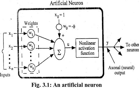
Artificial neural systems, or neural networks (NN), are physical cellular systems, which can acquire, store, and utilize experiential knowledge. The knowledge is in the form of stable states or mappings embedded in networks that can be recalled in response to the presentation cues. Neural network processing typically involves dealing with large-scale problems in terms of dimensionality, amount of data handled, and the volume of simulation or neural hardware processing. This large-scale approach is both essential and typical for real-life applications. By keeping view of all these, the research community has made an effort in designing and implementing the various neural network models for different applications.Fig. 3.1: An artificial neuron
The artificial neuron is developed to mimic the first-order characteristics of the biological neuron. In similar to the biological neuron, the artificial neuron receives many inputs representing the output of other
neurons. Each input is multiplied by a corresponding weight, analogous to the synaptic strength. All of these weighted inputs are then summed and passed through an activation function to determine the neuron input. This artificial neuron model is shown in Fig.3.1.
The mathematical model of the artificial neuron may written as
u(t) = w1x1 + w2x2 + w3x3+ . . . + wnxn
=
n
i i i
x
w
1θ
=
n
i i i
x
w
0 (3.1)
Assuming w0 = - and x0 = 1
y(t) = f [u(t)]
(3.2) where f[.] is a nonlinear function called as the activation function, the input-output function or the transfer function. In equation (3.1) and Fig.3.1, [x0, x1… xn] represent the
inputs, [w0, w1. . . . wn] represents the corresponding
synaptic weights. In vector form, we can represent the neural inputs and the synaptic weights as
X = [x0, x1… xn]T , and W = [w0, w1, . . . . , wn]
Equations (2.1) and (2.2) can be represented in vector form as:
U = WX
(3.3) Y = f[U]
(3.4) The activation function f[.] is chosen as a nonlinear function to emulate the nonlinear behavior of conduction current mechanism in biological neuron. The behavior of the artificial neuron depends both on the weights and the activation function. Sigmoidal functions are the commonly used activation functions in multi-layer static neural networks
In general the training of any artificial neural network has to use one of the following basic learning mechanisms.
The basic learning mechanisms of neural networks are:
i. Error-correction learning, ii. Memory-based learning, iii. Hebbian learning, iv. Competitive learning and
v. Boltzmann learning.
approach is that the domain knowledge is distributed in the neurons and information processing is carried out in parallel-distributed manner. Being adaptive units, they are able to learn these complex relationships even when no functional model exists. This provides the capability to do ‘Black Box Modeling’ with little or no prior knowledge of the function itself. ANNs have the ability to properly classify a highly non-linear relationship and once trained, they can classify new data much faster than it would be possible by solving the model analytically. The rising interest in ANNs is largely due to the emergence of powerful new methods as well as to the availability of computational power suitable for simulation. The field is particularly exciting today because ANN algorithms and architectures can be implemented in VLSI technology for real-time applications.
The application of ANNs in many areas under electrical power systems has led to acceptable results.
IV. SIMULATION RESULTS
In this Chapter, one area and three area power system model of simulation results are presented. In order to verify the proposed topology, matlab simulation is carried out.
The block diagram for single-area power system is shown in Fig. 4.1.
FREQ
2
PI
1
f1 1
10s+1 1
0.3s+1
ACE Out1
Out2
Subsystem1
Out1
Subsystem
deltaf1
Goto 20
0.4
1
0.1s+1
Fig.4.1: Simulink Block-diagram of a single-area power system model
Fig.4.2: Schematic diagram of the i th area model in the multi-area LFC system
Simulation results of a single area and multi area is considered in this section to analyze the efficiency of proposed system. The applied disturbances in the load model are shown in Fig.4.3.
0 20 40 60 80 100 120
0 0.01 0.02 0.03 0.04 0.05 0.06
Time (s)
D
el
ta
P
d
Fig.4.3: Load disturbances applied in Fig.4.1.
0 20 40 60 80 100 120
-3 -2 -1 0 1 2 3 4x 10
-3
Time (sec)
D
el
t
a
f
Fig.4.4: System frequency deviation with the Event triggered PI-ADP, traditional PI-ADP and Event
Triggerd PI control in area power system
0 20 40 60 80 100 120
-0.04 -0.02 0 0.02 0.04 0.06 0.08
Time (sec)
U
p
i
Event-triggered PI-ADP Traditional PI-ADP Event-triggered PI
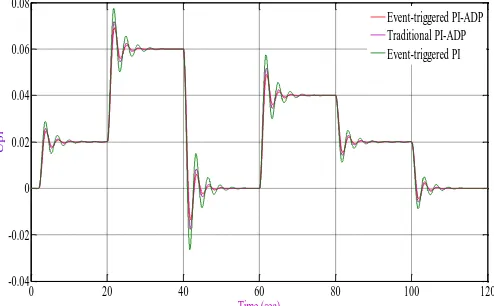
Fig.4.4: PI output with the Event triggered PI-ADP, traditional PI-ADP and event-triggered PI control in
one-area power system
0 20 40 60 80 100 120
-6 -4 -2 0 2 4x 10
-4
Time (sec)
U
ad
p
Event-triggered PI-ADP Traditional PI-ADP
Fig.4.5: ADP output with Event triggered PI-ADP and traditional PI-ADP
0 40 80 120
0 1 2
x 10-4
Time (s)
erro
r
Event Triggered error Threshold
Fig.4.6: illustration of event triggered error and threshold of one area power system
Fig. 4.3 shows the dynamics of the one area power system. In this it shows that the proposed method is effective when compared to event triggered and traditional PI-ADP. The output of PI controller of three different control methods is shown in Fig.4.4. ADP output with traditional PI-ADP and proposed event PI-ADP method is shown in Fig.4.5. The comparison between threshold and the event triggered error of proposed method is shown in Fig.4.6.
The parameters used in the test system are presented in Table 4.1.
0
50
100
150
-6
-4
-2
0
2
4
x 10
-3
Time (sec)
d
el
t
af1
Event triggered PI-ADP
Traditional ADP
Event triggered PI
0 50 100 150
-6 -4 -2 0 2 4x 10
-3
Time (sec)
d
el
t
af2
Event triggered PI-ADP Traditional ADP Event triggered PI
0 50 100 150
-6 -4 -2 0 2 4x 10
-3
Time (sec)
d
el
t
af3
Event triggered PI-ADP Traditional ADP Event triggered PI
Fig.4.7: Illustration of load frequency deviation of 3-area power system
0 50 100 150
0 1 2 3 4 5 6x 10
-3
Time (sec)
erro
r Event triggered error
Threshold
Fig.4.8: Illustration of event triggered error and threshold of 3-area power system
0 50 100 150
-0.3 -0.2 -0.1 0 0.1 0.2 0.3 0.4
Time (s)
W
ei
g
h
ts
o
f
A
ct
io
n
N
et
w
o
rk
Wa(1) Wa(2) Wa(3) Wa(4) Wa(5) Wa(6) Wa(7) Wa(8) Wa(9)
Fig.4.9: Learning weights of the action network for 3-area power system
system with proposed method in comparison with event triggered PI control and traditional PI-ADP is shown in Fig.4.7. The proposed method illustrated the good response and stabilized within the less time. The illustration of threshold and event triggered PI-ADP is shown in Fig.4.8. The learning weights of the action network for three area power system are shown in Fig.4.9.
0 50 100 150
-2 0 2 4 6
Time (sec)
J
V
A
L
U
E
(a)
0 50 100 150
-0.4 -0.2 0
Time (sec)
U
t
i
l
i
t
y
fu
n
ct
i
o
n
(b)
Fig.4.10: (a) J-value and (b) Utility function of 3-area power system
In the proposed event-triggered PI controller, weights of action network and the integral action are updated if the thresholds are exceeded. Therefore it reduces the calculation time and cost significantly.
V.
CONCLUSION
In this thesis, an event-triggered method for LFC system with PI and supplementary ADP control is
proposed. The proportional and integral actions of the PI controller used different thresholds for communication transmission, while the ADP controller with the actor-critic framework provided the supplementary signal for the PI controller in an aperiodic manner. By using the proposed design, the unnecessary events transmission was prevented. The comparative studies conducted demonstrated the proposed method could significantly save the computation cost without loss of control performance.
The proposed event-triggered scheme by considering the signal transmission delay and packet drop will be possible for future work.
VI. REFERENCES
[1]. H. Bevrani, Robust Power System Frequency Control. New York, NY, USA: Springer, 2009.
[2]. G. Gross and J. W. Lee, “Analysis of load frequency control performance assessment criteria,” IEEE Trans.
Power Syst., vol. 16, no. 3, pp. 520–525, Aug. 2001.
[3]. P. Mercier, R. Cherkaoui, and A. Oudalov, “Optimizing a battery energy storage system for frequency control application in an isolated power system,” IEEE Trans. Power Syst., vol. 24, no. 3, pp. 1469–1477, Aug. 2009.
[4]. H. Shayeghi, H. A. Shayanfar, and A. Jalili, “Load frequency control strategies: A state-of-the-art survey for the researcher,” Energy Convers. Manage., vol. 50, no. 2, pp. 344–353, 2009.
[5]. I. P. Kumar and D. P. Kothari, “Recent philosophies of automatic generation control strategies in power systems,” IEEE Trans. Power Syst., vol. 20, no. 1, pp. 346–357, Feb. 2005.
[6]. S. Pandey, S. R. Mohanty, and N. Kishor, “A literature survey on load frequency control for conventional and distribution generation power systems,” Renew. Sustain. Energy Rev., vol. 25, pp. 318–334, 2013.
[7]. D. Rerkpreedapong, A. Hasanovic, and A. Feliachi, “Robust load frequency control using genetic algorithms and linear matrix inequalities,” IEEE
Trans. Power Syst., vol. 18, no. 2, pp. 855–861, May
2003.
communication delays,” IEEE Trans.Power Syst., vol. 19, no. 3, pp. 1505–1515, Aug. 2004.
[9]. E. Cam and I. Kocaarslan, “Load frequency control in two area power systems using fuzzy logic controller,”
Energy Convers. Manage., vol. 46, no. 2, pp. 233–
243, 2005.
[10]. K. Vrdoljak, N. Peric, and I. Petrovic, “Sliding mode based load-frequency control in power systems,”
Elect. Power Syst. Res., vol. 80, no.5, pp. 514–527,
2010.
[11]. S. Saxena and Y. V. Hote, “Load frequency control in power systems via internal model control scheme and model-order reduction,” IEEE Trans. Power Syst., vol. 28, no. 3, pp. 2749–2757, Aug. 2013.
[12]. S. Vachirasricirikul and I. Ngamroo, “Robust LFC in a smart grid with wind power penetration by coordinated V2G control and frequency controller,”
IEEE Trans. Smart Grid, vol. 5, no. 1, pp. 371–380,
Jan.2014.
[13]. V. Ganesh, K. Vasu, and P. Bhavana, “LQR based load frequency controller for two area power system,”
Int. J. Adv. Res. Electr., Electron., Instrum. Eng., vol.
1, no. 4, pp. 262–269, 2012.
[14]. S. Mohagheghi, G. K. Venayagamoorthy, and R. G. Harley, “Adaptive critic design based neuro-fuzzy controller for a static compensator in a multimachine power system,” IEEE Trans. Power Syst., vol. 24, no. 1, pp. 1744–1754, Feb. 2006.
[15]. W. Guo, F. Liu, J. Si, D. He, R. Harley, and S. Mei, “Approximate dynamic programming based supplementary reactive power control for DFIG wind farm to enhance power system stability,”
Neurocomputing, vol. 170, pp. 417–427, 2015.
[16]. Y. Tang, J. Yang, J. Yan, Z. Zeng, and H. He, “Intelligent load frequency controller using GrADP for island smart grid with electric vehicles and renewable resources,” Neurocomputing, vol. 170, pp.406–416, 2015
[17]. W. Heemels, M. Donkers, and A. R. Teel, “Periodic event-triggered control for linear systems,” IEEE
Trans. Autom. Control, vol. 58, no.4, pp. 847–861,
Apr. 2013.
[18]. W. Heemels, J. H. Sandee, and P. Van Den Bosch, “Analysis of event driven controllers for linear systems,” Int. J. Control, vol. 81, no. 4, pp.571–590, 2008.