The In-and-Out-of-Sample (IOS) Likelihood Ratio
Test for Model Misspecification
Brett Presnell and Dennis D. Boos∗
Abstract
A new test of model misspecification, based on the ratio of in-sample and out-of-sample likelihoods, is proposed. The test is broadly applicable, and in simple problems approximates well known, intuitive methods. Using jackknife influence curve approxima-tions, it is shown that the test statistic can be viewed asymptotically as a multiplicative contrast between two estimates of the information matrix that are equal under correct model specification. This approximation is used to show that the statistic is asymp-totically normally distributed, though it is suggested that p-values be computed using the parametric bootstrap. The resulting methodology is demonstrated with a variety of examples and simulations involving both discrete and continuous data.
KEY WORDS: Goodness of fit; lack of fit; cross-validation; jackknife; parametric boot-strap; generalized linear model; sandwich matrix.
Institute of Statistics Mimeo Series No. 2536 August 2002
∗Brett Presnell is Associate Professor, Department of Statistics, University of Florida, Gainesville, FL
1
Introduction
1.1 Motivation
Model misspecification is always a concern when statistical inferences are based on a para-metric likelihood. Even when a model manages to capture the gross features of the data, misspecification of distributional forms, dependence structures, link functions, and other “structural” components of the model can cause estimates to be biased and their precision to be misrepresented. Other inferences based on likelihood are similarly affected, including tests of nested hypotheses within the model.
These concerns have led to a long and continuing history of “specification tests” in the econometrics literature, beginning with Hausman (1978) and White (1982). The statistics literature too has seen a renewed interest in general methods for testing model adequacy, as exemplified by Bayarri and Berger (2000) and Robins, van der Vaart and Ventura (2000).
Nevertheless, a useful general approach to testing for model misspecification is hard to find. A major difficulty is that there is often no obvious way to embed distributional assump-tions and other structural components of the assumed model into a larger model, with the aim of treating this larger model as the “full model” and the assumed model as the “reduced model” in a comparison of nested models. With categorical data, the “saturated model” can sometimes play the role of the larger model (see Agresti, 2002, pp. 139–141), but not when there are continuous predictors or otherwise too many settings of explanatory variables. For continuous data, no such approach is generally available.
To overcome these difficulties, we suggest comparing the maximized model likelihood to a corresponding “likelihood” motivated by cross-validation. To set notation, let Y1, . . . , Yn be
independent random variables with hypothesized densities f(y;xi, θ), where xi is a possible
predictor forYi and θis an unknownp-dimensional parameter. Note thatYi may be discrete
(in which case its density might be called a probability mass function), that both Yi and
xi may be vector valued, and that we take the xi to be nonrandom, so that our analysis
is conditional on the values of any predictors. Let θbbe the maximum likelihood estimator (MLE) ofθ, and letθb(i) be the MLE when the ith observation is deleted from the sample.
To motivate our test statistic, note thatf(Yi;xi,bθ(i)), the estimated likelihood ofYi given
the model and the remaining data, is a measure of how well the model is able to predict the
ith observation. In particular, iff(Yi;xi,bθ) is much larger thanf(Yi;xi,θb(i)), then the fitted model must shift appreciably in order to accommodate theith observation, suggesting that the model is in some way inadequate to describe the data. This leads us to compare the ordinary maximized, or “in-sample” likelihood,Qni=1f(Yi;xi,bθ), with the cross-validated, or
ratio,
IOS = log
Qn
i=1f(Yi;xi,θb)
Qn
i=1f(Yi;xi,θb(i))
! = n X i=1
l(Yi;xi,θb)−l(Yi;xi,θb(i)) , (1)
wherel(Yi;xi, θ) = logf(Yi;xi, θ). Note that IOS is always nonnegative, because n
X
j=1
l(Yj;xj,θb(i))−l(Yi;xi,θb(i))≥
n
X
j=1
l(Yj;xj,θb)−l(Yi;xi,bθ) by definition ofθb(i)
≥
n
X
j=1
l(Yj;xj,θb(i))−l(Yi;xi,θb) by definition ofθb,
which implies thatl(Yi;xi,θb)≥l(Yi;xi,θb(i)) for all i= 1, . . . , n.
1.2 Some Simple Examples
In simple cases, the IOS statistic often approximates well-known, intuitive statistics, as seen in the following examples.
Example 1 (Poisson Distribution). The assumed probability mass function is f(y;λ) =
e−λλy/y! with log likelihood −nλ+Pni=1Yilog(λ)−Pni=1log(Yi!) maximized atλb=Y, the
sample mean. Then
IOS =
n
X
i=1
(Y(i)−Y) +
n
X
i=1
Yilog(Y /Y(i))≈
s2 Y,
wheres2 is P(Yi−Y2)/(n−1) and we have used the fact that Y(i)−Y = (Y −Yi)/(n−1)
and the Taylor expansion log(Y(i)) ≈log(Y) + (Y(i)−Y)/Y. Of course s2/Y is the familiar Fisher (1973, p. 58) statistic (divided by n−1) for testing goodness of fit for the Poisson distribution.
Example 2 (Exponential Distribution.). The assumed density isf(y;σ) = exp(−y/σ)/σ
with log likelihood−Pni=1Yi/σ−nlog(σ) maximized atσb=Y. Then
IOS = n X i=1 Yi 1
Y(i) − 1 Y − n X i=1
log(Y /Y(i))≈
s2
Y2,
using approximations as in the previous example. Here again we see an obvious comparison of sample moments motivated by the exponential moment relationship var(Yi) ={E(Yi)}2.
Example 3 (Normal Distribution). The assumed density is f(y;µ, σ) = exp{−(y − µ)2/2σ2}/√2πσ with MLE’sµb=Y andσb2 =P(Y
i−Y)2/n. Somewhat lengthy calculations
lead to
IOS≈ 1 2
b
µ4
b
σ4 + 1
wherebµ4 =Pni=1(Yi−Y)4/n.It may seem surprising that, in the limit, the IOS statistic for
normality depends only on sample kurtosis and not on sample skewness, but as we look at the in-probability limit of the statistic below, the technical reason becomes clear. Note that under normality, the sample kurtosis converges in probability to 3 and IOS→P 2 as n→ ∞.
Example 4 (Normal Regression through the Origin.). The assumed density is normal with meanβxi and varianceσ2, where Pni=1xi = 0. The approximate version of IOS given
in Section 2 leads to
IOS≈
Pn
i=1be2ix2i
b
σ2Pn
i=1x2i
+ 1 2
b
µ4
b
σ4 + 1
,
whereβb=Pni=1Yixi/Pni=1x2i,ebi =Yi−βxb i,bσ2=n−1Pni=1be2i, andµb4=n−1Pni=1be4i. Thus
IOS retains the kurtosis term but adds a term that is related to the linear model specification, especially the homogeneity of errors assumption (cf. White, 1980).
Under the null hypothesis of correct model specification, the IOS statistic in each of these examples converges in probability to p, the dimension of the parameter vector θ. This is no accident. To see why, consider the case of independent and identically distributed (iid)
Y1, . . . , Yn with no predictors. Let I(θ) = E{−¨l(Y1;θ)} and B(θ) = E{l˙(Y1;θ)˙l(Y1;θ)T}, where ˙l(y;θ) = ∂l(y;θ)/∂θ, the p×1 gradient vector of partial derivatives of l(y;θ) with respect to the elements of θ, and where ¨l(y;θ) = ∂2l(y;θ)/∂θ∂θT, the p×p Hessian matrix of second-order partial derivatives. Finally, let θ0 represent the in-probability limit of θb, assumed to exist even when f(y;θ) is not correctly specified. Then Theorems 2 and 4 of Section 4 imply that under suitable regularity conditions,
IOS→P IOS∞=El˙(Y1;θ0)TI(θ0)−1l˙(Y1;θ0) = trI(θ0)−1B(θ0) (2)
asn→ ∞, where tr(A) denotes the trace of a matrixA. Of course under correct specification,
I(θ0) =B(θ0) and IOS∞=p, the trace of the p-dimensional identity matrix.
In typical situations where the model is misspecified, IOS∞ > p, but this is not always
the case. For example, in the iid Normal model of Example 3, IOS∞= (µ4/µ22+ 1)/2, where
µk=E
{Y1−E(Y1)}k
, so that IOS∞ < p= 2 whenever the true distribution has kurtosis
µ4/µ22 < 3, i.e., whenever the tails of the distribution are lighter than those of the normal distribution.
1.3 Links with Other Methods
Equation (2) suggests a connection between IOS and the Information Matrix (IM) Test of White (1982). The IM test is based on a quadratic form in the vector of differences between elements ofBb(θb) =n−1Pni=1l˙(Yi;θb)˙l(Yi;θb)T and the (average) observed information matrix
b
I(θb) = n−1Pn
i=1{−¨l(Yi;θb)}. Thus the IM test works by differencing two estimates of the
the other hand, as we show in Section 4, IOS can be approximated for large samples by trbI(θb)−1Bb(θb) , which is effectively a matrix ratio of two estimates of the Fisher information. This approximate form provides another motivation for IOS. Recall that when the dis-tributional form of the model is incorrectly specified, it still may be possible to carry out (asymptotically) valid inference using a sandwich estimator of the covariance matrix of θb, though generally with some loss in efficiency if the parametric model happens to be correct. By contrasting the model dependent estimate, Ib(θb), of var{l˙(Y1;θ0)} with the empirical es-timate, Bb(θb), IOS, like the IM Test, can indicate situations where model-based inference is invalid.
Of course the IOS test differs from the IM test in important ways. IOS is defined directly in terms of the likelihood, and is easily motivated and understood without any reference to asymptotic arguments. Calculation of IOS is very similar to the computation of a jackknife bias or variance estimator. This can be computationally intensive, particularly for large sample sizes and particularly after embedding in a bootstrap loop, but the computations are easy given a reliable routine for calculating the MLE. Moreover, if the routine uses numerical derivatives, then no analytical expressions are required for even first derivatives of the log-density. For large sample sizes, the approximate form of IOS can be used and is also relatively straightforward to calculate, though second derivatives of the log-likelihood are required.
Computation of the IM test statistic is less automatic. A number of different forms of the IM statistic have been suggested, all requiring at least second order partial derivatives, and for some forms third order derivatives of the log-likelihood (see Horowitz, 1994, for references and further details). One must also be careful to remove any structural zeros and linear dependencies in the elements of the differenced information matrix estimates. Thus, though there are undoubtedly situations in which the IM test will have greater power than the IOS test, in general IOS is simpler to use.
IOS has connections to a variety of model selection procedures as well. Stone (1977) gives a heuristic derivation of (2) and shows that when the model is correctly specified, the out-of-sample log-likelihood is asymptotically equivalent to Akaike’s (1973) information criterion. Linhart and Zucchini (1986) also discuss use of the out-of-sample log-likelihood as a model selection criterion. The approximate form of IOS, trbI(θb)−1Bb(θb) , arises as the “trace term” in the asymptotic model selection criterion of Linhart and Zucchini (1986, Section 4.1.1), and examples discussed there include the Poisson and normal examples above.
the PSR quasi-Bayes criterion.
In these references, the out-of-sample likelihood is considered solely for model selection; that is, for choosing between two or more competing models. It is not compared to the in-sample likelihood or employed in any other way to test for model misspecification. Geisser (1989, 1990) uses Bayesian analogues of the individual IOS factors,f(Yi;xi,θb)/f(Yi;xi,θb(i)), to identify outlying, or “discordant” observations. This is perhaps closer in spirit to the IOS test, but is distinguished by the Bayesian emphasis and more importantly by the focus on discerning individual discordant observations as opposed to measuring model adequacy in a global way.
We emphasize here that we do not propose to use IOS as a model selection tool in the usual sense of choosing variables for inclusion in a model, nor do we intend or expect IOS to usurp the role of the likelihood ratio test and its usual competitors in comparing nested models. IOS is useful for testing the fit of the of the final model selected in such a comparison, or perhaps of the largest model under consideration, but a more narrowly focused test should nearly always have greater power in a nested comparison. Indeed, in many situations IOS may have no power whatsoever to detect that an important variable has been excluded from the model.
In the remainder of this paper we investigate the IOS test from both a practical and a theoretical viewpoint. Section 2 provides an overview of technical results, with further details postponed to Section 4. In Section 3 we illustrate this procedure with a number of examples, and provide the results of several small simulation studies of the size and power of the test in settings motivated by the examples. Finally, in Section 5, we summarize our findings and discuss possible extensions of the IOS test to other settings, including dependent data models and partial likelihood.
2
Overview of Theoretical Results
In this section we provide an overview of theoretical results concerning IOS, with precise statements of theorems and their proofs postponed until Section 4. To simplify the statements of theorems and their proofs, we restrict attention to the case of iid random vectors,Y1, . . . , Yn.
The asymptotic form of the IOS statistic is
IOSA= 1
n
n
X
i=1 ˙
l(Yi;θb)TIb(θb)−1l˙(Yi;θb) = trbI(θb)−1Bb(θb) .
In Section 4, we prove the following results:
Theorem 2: IOSA→P IOS∞, where IOS∞is defined in (2). Theorem 3: IOSA is asymptotically normally distributed.
Theorem 4: IOS−IOSA= op(n−1/2), and thus the conclusions of Theorems 2 and 3 also
apply to IOS.
The form of the asymptotic variance of IOS, derived in the appendix, is fairly complicated for routine use. Moreover, examples like the sample kurtosis in Example 3 indicate that the convergence to normality is slow. Thus we suggest that p-values be obtained via the para-metric bootstrap under the hypothesized model (Horowitz, 1994, makes the same suggestion for the IM test). Theorem 1 implies that in location-scale models these p-values are exact up to Monte Carlo error. More generally, the p-values are asymptotically uniform under the hypothesized model, and simulations indicate that they are quite accurate in small samples as well.
Clearly the approximation of IOS by IOSAis critical to our results. IOSAarises naturally from Taylor expansion of the log-density aboutθb,
l(Yi;θb(i)) =l(Yi;θb) + ˙l(Yi;θb)T(θb(i)−θb) + 1
2(θb(i)−bθ)
T¨l(Y
i;θei)(θb(i)−bθ), (3)
whereθei lies between bθ(i) andθb, and from the influence curve approximation
b
θ(i)−θb=− 1
nIb(bθ)
−1l˙(Y
i;θb) +Rni. (4)
Substituting (3) and (4) into the definition (1) of the IOS statistic, we have
IOS =−
n
X
i=1 ˙
l(Yi;θb)T(θb(i)−θb)− 1 2
n
X
i=1
(θb(i)−θb)T¨l(Yi;θei)(θb(i)−θb)
= IOSA−
n
X
i=1 ˙
l(Yi;θb)TRni−1
2
n
X
i=1
(θb(i)−θb)T¨l(Yi;θei)(θb(i)−θb). (5)
The influence curve approximation (4) is the key to developing the approximation of IOS by IOSA, and deserves further discussion here. It is easily shown that whenever the MLE is the sample mean, Y, then
b
θ(i)−θb=Y(i)−Y =− 1
n−1(Yi−Y) =− 1
n−1Ib(θb)
−1l˙(Y
i;θb).
Thus (4) is exact in this case, with Rni = 0, if we replace the factor 1/n by 1/(n−1).
More generally, (4) arises from Taylor expansion of the estimating equation forθb(i):
0 =X
j6=i
˙
l(Yj;θb(i)) =
X
j6=i
˙
l(Yj;θb) +
X
j6=i
¨
l(Yj; ˇθi)(θb(i)−θb)
=−l˙(Yi;θb(i))−nIb(θb)(θb(i)−θb)−
X
j6=i
−¨l(Yj; ˇθi) −nIb(θb)
(θb(i)−θb), (6)
where ˇθi lies between θb(i) and θb. Here we have used the fact that Pj6=il˙(Yj;θb) =−l˙(Yi;θb),
which follows from the estimating equation forθb. Equation (6) implies that
b
θ(i)−bθ=−1
nIb(θb)
−1l˙(Y
i;θb)−Ib(θb)−1Wni(θb(i)−θb), (7) where
Wni =
1
n
X
j6=i
−¨l(Yj; ˇθi)−Ib(θb), (8)
and from this (4) follows with
Rni =−Ib(θb)−1Wni(θb(i)−θb). (9)
A subtle but important detail is the use ofIb(θb) instead ofI(θb) in the approximation. This is necessary in order to obtain√nmax1≤i≤n
(Wni)kl
P
→0, which in turn is needed to prove in Theorem 4 that IOS and IOSAdiffer only byop(n−1/2).
3
Examples and Simulations
The examples in this section demonstrate application of the IOS test in a variety of settings. Simulation results are also given, investigating the size and power of the IOS test in settings motivated by the examples. All computations were done using the R system for statistical computation and graphics (Ihaka and Gentleman, 1996).
As discussed previously, we use parametric bootstrap p-values. In most of the examples we have used 4000 bootstrap samples to estimate bootstrap p-values, as this gives adequate accuracy for almost any purpose. In order to reduce computation times, we have generally used fewer bootstrap samples in our simulation studies. However, the minimum number of bootstrap samples used is 199, so that the accuracy of our estimates of test size and power is not too seriously affected (see Boos and Zhang, 2000, for details).
3.1 A Simple Gamma Example
Table 1: Maximum 24 hour precipitation for 36 inland hurricanes (1900–1969).
31.00 2.82 3.98 4.02 9.50 4.50 11.40 10.71 6.31 4.95 5.64 5.51 13.40 9.72 6.47 10.16 4.21 11.60 4.75 6.85 6.25 3.42 11.80 0.80 3.69 3.10 22.22 7.43 5.00 4.58 4.46 8.00 3.73 3.50 6.20 0.67
Mountains in the period from 1900 to 1969. Larsen and Marx (2001) use the method of moments to fit a gamma distribution to these data.
Is the gamma model appropriate? The IOS test suggests not, with IOS = 3.60 for this two parameter model, giving an (estimated) bootstrap p-value of.028 based on 4000 bootstrap samples. For this example the IOSAstatistic takes the value IOSA= 2.84. Though this value does not seem particularly close to IOS, the bootstrap p-value is .022, in good agreement with the IOS p-value. For comparison, we also computed the Anderson-Darling statistic (.789) and the Kolmogorov-Smirnov statistic (.116), for which the bootstrap p-values were
.044 and .274, respectively. Thus, of these tests, the IOS tests give the strongest evidence against the gamma model, with the Anderson-Darling test in reasonably close agreement. The Kolmogorov-Smirnov fails to find any evidence against the gamma model in this example.
The observations 31.00, 0.67, 22.22, and 0.80 make the largest contributions to IOS, 1.73, 0.49, 0.45, and 0.38 respectively. After deletion of the largest observation, 31.00, the IOS and IOSAtests still yield mild evidence against a gamma model for the remaining data, with bootstrap p-values of.061 and.053, respectively, while the p-value for the Anderson-Darling test increases to.164.
3.1.1 Simulation
To examine the size of the IOS test in this context, we ran a small simulation with 4000 samples of size 36 drawn from a gamma distribution with shape parameter 2.187 equal to the maximum likelihood estimate for the rainfall data. For each sample, bootstrap p-values for the Anderson-Darling, the Kolmogorov-Smirnov, the IOS, and the IOSAtests were estimated using 199 bootstrap samples. The estimated size of the nominal .05 level tests were .049, 0.055, 0.047, and 0.047, respectively, all well within simulation error of.05.
3.2 Leukemia Survival Times
Feigl and Zelen (1965) applied an exponential regression model (with identity link) to the survival times of thirty-three leukemia patients, using the logarithm of white blood count (WBC) and a binary factor (AG) as predictors. Patients were identified as AG positive by the presence of Auer rods and/or significant granulature of leukemic cells at diagnosis. There were 17 AG positive and 16 AG negative patients.
survival distribution variously as gamma, Weibull, and lognormal (a Gaussian model fitted to log(time)). They found that the exponential (with log link) was very nearly the best fitting model within both the gamma and the Weibull families. Using graphical methods, they found no evidence of lack of fit for any of these models. Comparing maximized likelihoods, they stated that the lognormal provided a slightly better fit than the exponential/gamma/Weibull model, but they did not judge the difference to be significant.
We applied the IOS test to the gamma model with log link and to the lognormal model with identity link. The linear predictor included a WBC:AG interaction term, so that both models have five parameters to be estimated. For both models we used 4000 bootstrap replications to estimate the p-value for the IOS test.
For the gamma model, IOS = 15.74. For 10 of the bootstrap samples, calculation of either the full MLE or at least one of the 33 leave-one-out estimators failed. Of the remaining 3990 bootstrap samples, 125 yielded a value of the IOS statistic greater than the observed value. Thus the estimated p-value is about .031 (or conservatively, .034), and there is appreciable evidence against the gamma model. For the lognormal model, IOS = 7.29, and the estimated bootstrap p-value is.22, providing no evidence against the model.
Does it matter which model we use for these data? We think that it does. The lognormal model provides more precise estimates in this example than the gamma model rejected by the IOS test. For example, in the gamma model, the Wald test yields a p-value of .25 for the AG:WBC interaction. Thus, the data analyst might be inclined to drop this term from the model and declare that the slopes for the two AG groups are not significantly different. Indeed, this is one of the models suggested by Aitkin et al. (1989) in the exponential case. In the lognormal model, however, the Wald test yields a p-value of.08 for the interaction, so that the data analyst might think more carefully before dropping it.
Recognizing the interaction is important in this example. The slope for the AG negative group is not significantly different from 0 in either model (the p-value for the Wald test is
.48 in the gamma model and.34 in the lognormal model). Thus, for the AG negative group there appears to be at best a weak dependence of survival time on WBC, whereas in the AG positive group the relationship is significant. Indeed, this was perhaps the most important findings in the original analysis of Feigl and Zelen (1965). Though a careful data analyst might uncover this feature of the data with either the gamma or the lognormal model, there is a greater chance that it would go undetected if the gamma model were used.
3.2.1 Simulation
For 16 of the 400 simulated samples, we were unable to compute IOS either for the sample itself, or for at least one of the corresponding bootstrap samples. This may seem surprising, but for each simulated sample we must fit a gamma model both to the full data and to the 33 delete-one subsamples, and then repeat this procedure 199 times for the bootstrap samples. Thus we must compute maximum likelihood estimates for the gamma model for a total of 34×200 = 6800 data sets for each simulated sample. Maximum likelihood estimation of the regression and shape parameters of a gamma model is not so stable that this process can always be counted on to succeed without any human intervention. In practice, one can simply keep track of the number of bootstrap samples for which the computation of IOS failed and report a suitably adjusted p-value as we have done in the example, but for this small simulation we decided to simply discard these samples. Of the remaining 384 simulated samples, 23 yielded an estimated bootstrap p-value less than.05. Thus the estimated size of the IOS test is.06, well within simulation error of the nominal .05 level.
For the lognormal model, maximum likelihood estimates are more easily computed, and here we used 1599 bootstrap resamples to estimate bootstrap p-values for each of 400 samples generated from the fitted normal model. In this case 22 of the estimated p-values were less than.05, so that the estimated size of the IOS test is.055, again well within simulation error of the nominal.05 level.
Finally, because the IOS test fails to reject the lognormal model in this example, the power of the IOS test of this model is of interest. For the alternative we chose to use a gamma model, and so for each of 400 samples generated from the fitted gamma model, we computed IOS for an assumed lognormal model. For each sample we again used 1599 bootstrap resamples to estimate the bootstrap p-value of the test. The power of the.05 level test was thus estimated as 76/400 = .19. Of course it is difficult to say much about power on the basis of such a limited simulation, but with a five parameter regression model and a sample size of only 33, we judge this a reasonably positive performance, particularly given the dearth of competitors for the IOS test in this situation.
3.3 Drill Advance Rates
Table 2: Free throws by basketball player Shaquille O’Neal in 23 playoff games.
Game 1 2 3 4 5 6 7 8 9 10 11 12 13 14 15 16 17 18 19 20 21 22 23 Attempted 5 11 14 12 7 10 14 15 12 4 27 17 12 9 12 10 12 6 39 13 17 6 12 Made 4 5 5 5 2 7 6 9 4 1 3 5 6 9 7 3 8 1 8 3 0 1 3
bootstrap replications. For the gamma model, IOS = 8.37 with an estimated bootstrap p-value of .64. Thus IOS finds no evidence again either of these models. This is perhaps not surprising given the small sample size, but it does suggest that the use of either model is justifiable.
3.4 Testing Multivariate Normality
Johnson and Wichern (1998) examine a data set consisting of four different measurements of stiffness taken on each of 30 wooden boards. Although the four variables taken individually appear to be marginally normal, a plot of Mahalanobis distances from the mean against quantiles of a chi-square distribution with 4 degrees of freedom suggests that at least two of the observations may be multivariate outliers.
We applied the IOS test and Mardia’s multivariate skewness and kurtosis tests (see Mar-dia, Kent and Bibby, 1979, section 5.7) to these data. Under multivariate normality, the distribution of all three of these statistics is free of the unknown mean and covariance ma-trix, so that parametric bootstrap p-values are exact up to simulation error. For the 14 parameter multivariate normal model, IOS = 30.7, with a p-value of .002 based on 4000 bootstrap replications. The multivariate skewness and kurtosis were 7.54 and 30.42 with bootstrap p-values of.008 and .001, respectively.
Johnson and Wichern (1998) identify observations 9 and 16 as outliers based on their Mahalanobis distances. This is supported by their large contributions, 5.1 and 13.5, respec-tively, to IOS. With these two observations deleted, IOS = 27.2, with a p-value of.006 based on 4000 bootstrap replications. Results for the skewness and kurtosis tests were similar, with bootstrap p-values of .004 and .006, respectively. Thus there is still strong evidence of non-normality, even after deletion of the two presumed outliers.
We have applied these three tests to a number of data sets, and generally p-values for the IOS test agrees very closely with the kurtosis test. For large sample sizes, IOS and the multivariate kurtosis appear to be nearly linearly related, and we speculate that IOSA is indeed an affine function of Mardia’s multivariate kurtosis, although we have not verified this analytically.
3.5 A Simple Binomial Example
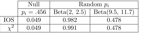
Table 3: Size and power of nominal .05 level IOS and chi-squared tests in the free throw shooting example.
Null Random pi
pi =.456 Beta(2, 2.5) Beta(9.5, 11.7)
IOS 0.049 0.982 0.478
χ2 0.049 0.991 0.478
player Shaquille O’Neal. We take as our null hypothesis that the Yi are independent
bino-mial random variables with common, unknown success probability. To test this hypothesis, Stefanski and Boos computed parametric bootstrap p-values for Pearson’s chi-squared statis-tic in the 23×2 table (which is the score statistic in this example). We re-ran their analysis using 100,000 bootstrap samples, with the ni fixed at their observed values for each game,
and obtained a p-value of .028 for the chi-squared test. (Note that the p-value reported by Stefanski and Boos (2002) are incorrect because of a programming error discovered after publication.) The IOS statistic, on the other hand, takes the value 1.29, with a bootstrap p-value of.206. This suggests that the IOS test may have much lower power than the score test in the setting of this example, though we suspect that the difference in p-values is largely due to a greater sensitivity of the chi-square test to the extreme observation in game 14, in which O’Neal made 9 of 9 free throw attempts. To explore this issue further, we carried out a small simulation study.
3.5.1 Simulation
In each simulation the number of attempts were fixed at the observed values, n1, . . . , n23. Bootstrap samples were also generated with the same fixed binomial sample sizes, so that all analysis is conditional on the number of attempts. P-values were computed using 1000 parametric bootstrap resamples. All results are based on 20,000 simulated samples.
To study the size of the tests, we generated samples using a constant success probability,
p = 0.456, equal to O’Neal’s overall free throw shooting percentage for the 23 games. The estimated sizes of the nominal.05 level tests, given in the first column of Table 3, are all well within probable simulation error of.05.
To study power, we let the success probabilitiespi, 1≤i≤23, vary independently from
game to game according to a beta distribution, with the Yi independent and binomially
distributed conditional on the pi. In the first simulation, we chose the parameters of the
beta distribution to match the (unweighted) mean and variance of O’Neal’s observed success probabilities over the 23 games, 0.45 and and 0.045, respectively. This corresponds to a beta distribution with parameters 2.0 and 2.5. Against this alternative, both the IOS and the chi-squared tests have power very close to 1, as shown in the fourth column of Table 3. To obtain a more informative comparison, we ran another simulation with beta distributed
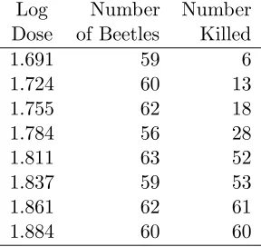
Table 4: Beetle mortality data (Bliss, 1935).
Log Number Number
Dose of Beetles Killed
1.691 59 6
1.724 60 13
1.755 62 18
1.784 56 28
1.811 63 52
1.837 59 53
1.861 62 61
1.884 60 60
corresponds to a beta distribution with parameters 9.5 and 11.7. The power of both the IOS and chi-squared tests against this alternative are moderate and nearly equal, as shown in the fifth column of Table 3. These results suggest that the power of the IOS test is comparable to that of the score test in this simple situation, though the latter may have greater power against a single extreme pi.
3.6 Beetle Mortality Data
Table 4, taken from Agresti (2002, p. 247), reports the number of beetles killed after five hours of exposure to eight different concentrations of gaseous carbon disulphide (these data were originally reported by Bliss, 1935). Agresti finds that a binomial model with complementary log-log link fits these data very well, and that the model with logit link fits poorly. Specifically, the residual deviances, 3.5 for the model with complementary log-log link and 11.1 for the model with logit link, yield p-values of .74 and .085, respectively, when referred to the chi-square distribution with 6 degrees of freedom.
The IOS statistic is 1.45 for the model with complementary log-log link, and 4.07 for the model with logit link. The corresponding bootstrap p-values, estimated with 4000 bootstrap samples, are .71 and .136, respectively. The p-value for the logit model suggests that IOS may be somewhat less sensitive here than the deviance statistic. However, for the two largest dose levels the fitted counts in these models are very close to the number of beetles tested, so that the chi-square approximation to the distribution of the deviance statistic may not be adequate. The parametric bootstrap p-value for the deviance test of the logit model.111, in much closer agreement with the IOS p-value.
3.7 Horseshoe Crab Satellites
model using the usual Pearson chi-square or residual deviance statistics, he is forced to pool the data over ranges of carapace width, and finds no evidence of lack-of-fit. Subsequently, however, he finds evidence of overdispersion, and prescribes adjustment of standard error estimates by an appropriate scaling factor.
Of course the continuous predictor is no hindrance to the IOS test. For this two parameter model, IOS = 5.55, suggesting a serious lack of fit, which is reinforced by the bootstrap: the estimated bootstrap p-value, based on 4000 bootstrap samples, was 0; the 99th percentile of the bootstrap IOS values was 3.20; only 5 of the 4000 bootstrap IOS values were greater than 4.0; and none were greater than 4.9.
For the negative binomial model with log link, IOS = 2.66. With 4000 bootstrap samples, the estimated p-value is.91, so there is no evidence against this model.
3.8 Testing Beta-Binomial Models
Binary data often exhibit overdispersion relative to a binomial model. Overdispersion may be caused, for example, by positive correlation of within litter responses in biological data. In such cases, beta-binomial models are often suggested as an alternative to the binomial (see Brooks, Morgan, Ridout and Pack, 1997; Slaton, Piegorsch and Durham, 2000).
Brooks et al. (1997) presented six data sets, labeled E1, E2, HS1, HS2, HS3, and AVSS, giving litters sizes and “success” counts for 205, 211, 524, 1328, 554, and 127 litters, re-spectively (Garren, Smith and Piegorsch, 2001, correct several errors in these data). Their analysis began by testing the goodness-of-fit of the beta-binomial distribution to each data set using the maximized likelihood as a test statistic. With this test they failed to find any evidence against the beta-binomial model for any of the six data sets. They then fitted sev-eral models to these data. In one particular model comparison, they found that for all but the AVSS data set, the beta-binomial model was significantly improved by a model mixing a beta-binomial distribution with a simple binomial component.
Garren, Smith and Piegorsch (2000) criticized Brooks, et al’s approach to testing goodness-of-fit for the beta-binomial model. In Garren et al. (2001) they proposed an alternative goodness-of-fit test based on pooling bootstrap p-values for Pearson chi-square statistics computed separately for each observed binomial sample sizen. Garren et al. (2001) applied their test to each of the six data sets from Brooks et al. (1997) and to three similar data sets taken from Lockhart, Piegorsch and Bishop (1992), with counts from 50, 201, and 263 litters, respectively. In what follows these data sets are labeled LPB(a), LPB(b), and LPB(c).
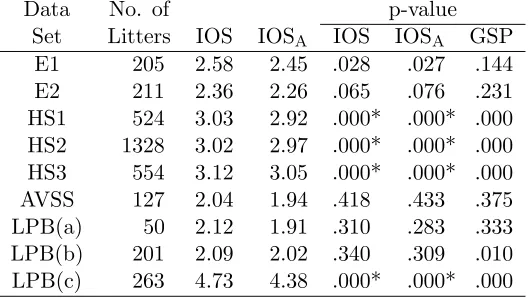
Table 5: Comparison of IOS, IOSA, and the test of Garren et al. (2001) for nine data sets.
Data No. of p-value
Set Litters IOS IOSA IOS IOSA GSP
E1 205 2.58 2.45 .028 .027 .144
E2 211 2.36 2.26 .065 .076 .231
HS1 524 3.03 2.92 .000* .000* .000
HS2 1328 3.02 2.97 .000* .000* .000
HS3 554 3.12 3.05 .000* .000* .000
AVSS 127 2.04 1.94 .418 .433 .375
LPB(a) 50 2.12 1.91 .310 .283 .333
LPB(b) 201 2.09 2.02 .340 .309 .010
LPB(c) 263 4.73 4.38 .000* .000* .000
* (No bootstrap IOS/IOSAexceeded observed value.)
The IOS and GSP tests agree except on all but the E1 and GSP(b) data sets, and perhaps the E2 data set. For the E1 data, the IOS test yields reasonably strong evidence against the beta-binomial model, whereas the GSP test does not. A more detailed examination of the terms of the IOS statistic reveals several observations that appear to contribute excessively to the observed value of IOS, including in particular a single observation, (n, y) = (14,9), that contributes 0.61. Recalculating IOS after removal of this observation yields an IOS value of 2.34, and a bootstrap p-value of .105 (again based on 400 bootstrap replications). For the LPB(b) data, the GSP test yields strong evidence against the beta-binomial model where IOS and IOSAfind none. Finally, for the E2 data set, the IOS test perhaps casts some doubt on the beta-binomial model, while the GSP test certainly does not.
Thus it appears that IOS and the GSP test perform similarly, although each test may be sensitive to alternatives to which the other is not. Of course the IOS test is based on a general approach to testing for model misspecification, whereas the GSP test seems to be useful only for testing simple binomial or beta-binomial models. In particular, while IOS can be used in an automatic way in regression settings, the GSP test does not seem to generalize in this direction, except perhaps in situations with heavily replicated design points.
As an example, we have applied the IOS test to the Heckman-Willis model used by Slaton et al. (2000) to analyze data from a dose response experiment. In this model, it is assumed that, conditional on the litter size, N, the number of “successes,” Y, in a litter follows a beta-binomial distribution, with parameters depending on the value of the predictor
x= dose. More precisely, it is assumed that Y has probability mass function
f(y|x) =
N y
Γ(α+β)Γ(α+y)Γ(β+N −y)
Γ(α)Γ(β)Γ(α+β+N) , y= 0, . . . , N,
where
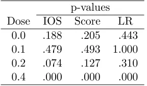
Table 6: P-values for three tests of the adequacy of separate binomial models for the four dose groups in the boric acid data. P-values for the IOS and score tests are based on 4000 bootstrap samples. The likelihood ratio test takes the beta-binomial as the larger model and uses the chi-square distribution with one degree of freedom as its reference distribution.
p-values
Dose IOS Score LR
0.0 .188 .205 .443
0.1 .479 .493 1.000
0.2 .074 .127 .310
0.4 .000 .000 .000
anda0,a1,b0, and b1 are unknown parameters to be estimated.
The data, given in Table 4 of Slaton et al. (2000), are from an experiment in developmental toxicology and consist of observations on 107 litters at four different dose levels of boric acid. For the four-parameter Heckman-Willis model, IOS = 6.34, with a bootstrap p-value of
.043 based on 400 bootstrap samples. For the asymptotic version of the test statistic, we observed IOSA = 5.19. In one of 4000 bootstrap samples the observed Fisher information matrix was numerically singular preventing calculation of IOSA. For 109 of the remaining 3999 bootstrap samples, the bootstrap value of IOSA exceeded the observed value, yielding an estimated bootstrap p-value of .027 (a conservative estimate of the bootstrap p-value is 110/4000 =.0275). Thus there is fairly strong evidence against the Heckman-Willis model for these data.
Slaton et al. (2000) used a likelihood ratio test to compare the the Heckman-Willis model with a more general beta-binomial model which shared with the Heckman-Willis model the logistic form of the mean as a function of dose, but which allowed the intralitter correlation to vary freely among the four different dose levels (thus they compared the four parameter Heckman-Willis model to a larger six parameter beta-binomial model). The resulting p-value of.32 indicated no departure from the Heckman-Willis model, but of course this test assumes that the larger model is correctly specified. Our analysis suggests otherwise.
Considering the four dose groups separately, the p-values given in Table 6 show little or no evidence against a binomial model for each of the first three dose levels (0, 0.1, and 0.2 percent boric acid in feed), while for the fourth dose group there is very strong evidence of extra-binomial variation. However, even the beta-binomial does not adequately describe the fourth dose group, as for this model IOS = 4.46, with an estimated p-value of .013 based on 400 bootstrap samples.
0.0 0.1 0.2 0.3 0.4
0.00
0.05
0.10
0.15
0.20
0.25
Dose
Overall Proportion Dead
Figure 1: Overall group proportions and fitted mean curve from Heckman-Willis model for boric acid data. Error bars represent two standard errors to either side of the overall proportion.
group. It seems clear that the logistic mean function is unable to accommodate the observed proportions, particularly for dose level 0.2.
4
Technical Results
In this section we provide detailed statements and proofs of the theoretical results outlined in Section 2. Unless otherwise specified,θ will be an unknownp-dimensional parameter vector belonging to a set Θ ⊂ Rp. The parametric models of interest have densities f(y;θ) with respect to some dominating measure, but we will not emphasize measure-theoretic aspects. Recall that we takel(y;θ) = logf(y;θ), ˙l(y;θ) =∂l(y;θ)/∂θ, and ¨l(y;θ) = ∂2l(y;θ)/∂θ∂θT.
The maximum likelihood estimator isθb, and we assume thatθbexists and solves the likelihood equationsPni=1l˙(Yi;θb) = 0. The matrix I(θ) = E{−¨l(Y1;θ)} will be called the information matrix even in cases where the assumed density is not the true density (misspecification), though it is more common to define the information matrix to beB(θ) =E{l˙(Y1;θ)˙l(Y1;θ)T}. Here and throughout this paper, expectations are taken with respect to the true underly-ing distribution of the Yi, which is not necessarily a member of the assumed model family
{f(y;θ) :θ∈Θ}. The (average) observed information matrix isIb(bθ) =n−1Pni=1−l¨(Yi;θb) ,
and we letBb(θb) =n−1Pni=1l˙(Yi;θb)˙l(Yi;θb)T. Finally,θ0 represents the in-probability limit of
b
θ, assumed to exist even whenf(y;θ) is not correctly specified.
For a vector x ∈ Rp, kxkr represents the Lr norm, i.e., kxkr = Ppi=1|xi|r
1/r
. The
Lr norm on Rp induces the r-norm on the space of p ×p matrices, defined by kAkr =
supkxkr=1kAxkr,A∈R
p×p (see Golub and van Loan, 1989, for details).
This first theorem shows that in location-scale models the distributions of IOS and IOSA do not depend on the true parameter values when the model is correctly specified. Thus the null distributions can be simulated exactly, and exact (up to simulation error) p-values can be obtained.
Theorem 1. Suppose that Y1, . . . , Yn are iid with location-scale density f(y;θ) =σ−1f0((y−
µ)/σ), where f0 is a known density with derivative f˙0(y) existing and such that the
maxi-mum likelihood estimator θb = (µ,b bσ)T exists and solves the likelihood equations. Then the
distributions of IOS and IOSA do not depend on the value of θ= (µ, σ)T.
Proof. For arbitrary real numbersa >0 andb, and dataY= (Y1, . . . , Yn), it is easy to show
thatµb(aY+b) =aµb(Y) +b,bσ(aY+b) =abσ(Y),l(ay+b;θb(aY+b)) =l(y;θb(Y))−log(a), ˙
l(ay+b;θb(aY+b)) =a−1l˙(y;bθ(Y)), and Iba
Y+b(θb(aY+b)) =a−2IbY(θb(Y)). It then follows
easily that IOS(aY+b) = IOS(Y) and IOSA(aY+b) = IOSA(Y).
The next theorem gives a consistency result for IOSA under both misspecified and cor-rectly specified models. Recall that expectations are taken with respect to the true under-lying distribution of theYi, which is not necessarily a member of the assumed model family
{f(y;θ) :θ∈Θ}.
Theorem 2. Let Y1, . . . , Yn be iid. Assume that l(y;θ) has three partial derivatives with
1. There existsθ0 such that θb→P θ0 as n→ ∞.
2. I(θ0) =E
−¨l(Y1;θ0) is finite and nonsingular.
3. B(θ0) =E
˙
l(Y1;θ0)˙l(Y1;θ0)T is finite.
4. There exists a functionC(y) such that for allθ in an open neighborhood of θ0 and for
all j, k, l∈ {1, . . . , p}, ∂¨l(y;θ)jk/∂θl
≤C(y),and E{C(Y1)}<∞.
5. There exists a function D(y) such that for all θ in an open neighborhood of θ0 and for
all j, k, l∈ {1, . . . , p}, ¨l(y;θ)jkl˙(y;θ)l
≤D(y), and E{D(Y1)}<∞.
Under the above conditions, IOSA→P IOS∞ as n→ ∞. Proof. Note that
bI(θb)jk−I(θ0)jk
≤ 1 n n X i=1
−¨l(Yi;θb)jk −
1 n n X i=1
−¨l(Yi;θ0)jk
+ 1 n n X i=1
−¨l(Yi;θ0)jk −I(θ0)jk
.
The second term is op(1) by the weak law of large numbers and Condition 2. By the mean
value theorem and Condition 1, the first term can be bounded with probability converging to 1 by n−1Pn
i=1C(Yi}
kθb−θk1, which, by Conditions 1 and 4 and the weak law of large numbers, isOp(1)·op(1) =op(1). ThusIb(θb) →P I(θ0) as n→ ∞. Using Conditions 3 and 5 in place of 2 and 4, a similar argument shows thatBb(θb) →P B(θ0) as n→ ∞. The theorem then follows from continuity of the trace and matrix inversion.
Remark 1. There is no loss of generality in the requirement that the bounding functionsC(y) andD(y) above do not depend onj,k, andl. If integrable bounding functions can found for each j, k, l combination, we can then take C(y) = maxj,k,lCjkl(y). The same remark applies
to Lemma 1 and Theorem 4 below.
The following general result will be applied in Theorem 3 to prove asymptotic normality of IOSA.
Lemma 1. Suppose thatY1, . . . , Yn are iid and assume that
1. The p×1 estimator θbhas an influence curve approximating function h(y;θ) such that
b
θ−θ0 = 1
n
n
X
i=1
h(Yi;θ0) +Rn1,
2. The real-valued functionq(Yi;θ) has two partial derivatives with respect toθ, and
(a) var{q(Y1;θ0)} and E{q˙(Y1;θ0)} are finite.
(b) there exists a function M(y) such that for all θ in a neighborhood of θ0 and all
j, k ∈ {1, . . . , p}, |q¨(y;θ)jk| ≤M(y), where E{M(Y1)}<∞.
Then 1 n n X i=1
q(Yi;θb)−E{q(Y1;θ0)}= 1
n
n
X
i=1
Q(Yi;θ0) +Rn2,
where Q(y;θ) =q(y;θ)−E{q(Y1;θ)}+E{q˙(Y1;θ)}Th(y;θ) and √nRn2→P 0 as n→ ∞, and
it follows that n−1Pn
i=1q(Yi;θb) is asymptotically normal with asymptotic mean E{q(Y1;θ0)}
and asymptotic variance var{Q(Y1;θ0)}/n.
Proof. By Taylor expansion and adding and subtracting terms, we have
1
n
n
X
i=1
q(Yi;θb) =
1 n n X i=1
q(Yi;θ0) +E{q˙(Y1;θ0)}Th(Yi;θ0)
+ 1 n n X i=1 ˙
q(Yi;θ0)−E{q˙(Y1;θ0)}
T
(θb−θ0)
+E{q˙(Y1;θ0)}T
b
θ−θ0− 1
n
n
X
i=1
h(Yi;θ0)
+1
2(θb−θ0)
T 1 n n X i=1 ¨
q(Yi;θe)
(bθ−θ0),
where θelies between θband θ0. Using Conditions 1 and 2 and the asymptotic normality of
b
θ that follows from Condition 1, it is straightforward to show that the last three terms are
op(n−1/2) asn→ ∞. The result then follows immediately from the central limit theorem.
The next theorem establishes the asymptotic normality of IOSA. Here vech represents the usual column stacking operator for symmetric matrices (see Harville, 1997, section 16.4).
Theorem 3. Let Y1, . . . , Yn be iid. Suppose that Condition 1 of Lemma 1 holds for the
maximum likelihood estimator bθ with h(y;θ0) = I(θ0)−1l˙(y;θ0), and that Condition 2 of
Lemma 1 holds for both q(y;θ) = −¨l(y;θ)jk and q(y;θ) = {l˙(y;θ)˙l(y;θ)T}jk for each j, k ∈
{1, . . . , p}. Then IOSAis asymptotically normal with asymptotic mean IOS∞ and asymptotic variance DTAD/n, where A/n is the asymptotic covariance matrix arising from the joint asymptotic normality of vech{Ib(θb)} and vech{Bb(bθ)}, and D is the p(p+ 1) dimensional vector of partial derivatives of IOSA taken with respect to the components of vech{Ib(θb)} and
Proof. Joint asymptotic normality of the elements of vech{Ib(θb)} and vech{Bb(θb)} follows from Lemma 1. The result then follows from a direct application of the delta method to IOSA= trbI(θb)−1Bb(bθ) .
The conditions onθbin Theorem 3 may be satisfied by modifications of the usual conditions for asymptotic normality ofθb(e.g., pages 462–463 of Lehmann and Casella, 1998) to allow for misspecification. Since the form of the asymptotic variance DTAD/n is fairly complicated, we defer further computations to the appendix.
Our last theorem establishes equivalence of IOS and IOSA to order op(n−1/2).
Theorem 4. Suppose that the conditions of Theorem 2 hold. Assume further that:
1. √nmax1≤i≤n
bθ(i)−θb2 →P 0 as n→ ∞.
2. There exists a functionG(y) such that for allθ in an open neighborhood of θ0 and for
all j∈ {1, . . . , p}, l˙(y;θ)j
≤G(y), and E{G(Y1)2}<∞.
3. There exists a function H(y) such that for all θ in an open neighborhood of θ0 and for
all j, k ∈ {1, . . . , p}, ¨l(y;θ)jk
≤H(y), and E{H(Y1)2}<∞.
Then
√
n(IOS−IOSA)→P 0 as n→ ∞.
If further, the conditions of Theorem 3 also hold, then IOS is asymptotically normal with asymptotic mean IOS∞ and asymptotic variance DTAD/n, whereDandA are as defined in Theorem 3.
Proof. The result will follow if we can show the two remainder terms in (5) are op(n−1/2).
Note that by Condition 1 of Theorem 2 and Condition 1 above, with probability tending to one, bθ, θb(i), and all values between θb(i) and θb, 1 ≤ i ≤ n, lie within the neighborhoods of
θ0 where the bounds in Conditions 4 and 5 of Theorem 2 and in Conditions 2 and 3 of the present theorem apply. In what follows, we will use these bounds freely without restating the qualifier that the resulting inequalities hold only with probability tending to one. This is permissible because we are concerned only with convergence in probability.
As mentioned in Section 2, a key quantity in the proof is the matrix Wni defined in (8).
By Taylor expansion, we have
(Wni)kl=
1 n n X j=1 ¨
l(Yj; ˇθi)kl−
1 n n X j=1 ¨
l(Yj;θb)kl−
1 n n X j=1 ¨
l(Yi; ˇθi)kl
= 1 n n X j=1 p X m=1
∂¨l(Yj;θ)kl
∂θm
θ=˜θ˜i
ˇ
θi−θb
m− 1 n n X j=1 ¨
where ˜θ˜i is between ˇθi and θb. Thus,
(Wni)kl
≤ p n n X j=1
C(Yj)· kθˇi−θbk2+ 1
nH(Yi),
by Condition 4 of Theorem 2 and by Condition 3. Now by Condition 1, and the assumptions
E{C(Y1)}<∞ and E{H(Y1)2}<∞, it follows that
√
n max
1≤i≤nkWnik2 ≤
p2
n
n
X
j=1
C(Yj)·√n max
1≤i≤nk
ˇ
θi−θbk2+ 1 √
n1max≤i≤nH(Yi)
=Op(1)op(1) +op(1)→P 0 (10)
asn→ ∞. Referring back to (9), this also implies that
n max
1≤i≤nkRnik2≤ kIb(θb)
−1
k2·√n max
1≤i≤nkWnik2·
√
n max
1≤i≤nkθb(i)−θbk2 P
→0. (11)
Addressing first the second remainder term in (5), recall from (7) and (9) that
b
θ(i)−θb=−1
nIb(bθ)
−1l˙(Y
i;θb) +Rni. (12)
Thus after some algebra, Conditions 1 and 3 and results (10) and (11) imply
√n n X i=1
(θb(i)−θb)T¨l(Yi;eθi)(θb(i)−θb)
≤bI(θb)−122 1
n3/2
n
X
i=1
l˙(Yi;θb)22¨l(Yi;θei)
2
+bI(θb)−12max 1≤i≤n
Rni 2 2
n1/2
n
X
i=1
l˙(Yi;bθ)
2
¨l(Yi;θei)
2
+max
1≤i≤n
Rni 2 2
n1/2
n
X
i=1
¨l(Yi;θei)
2
≤Op(1)
1
n3/2
n
X
i=1
G(Yi)2H(Yi) +op(1)
1
n3/2
n
X
i=1
G(Yi)H(Yi) +op(1)
1
n3/2
n
X
i=1
H(Yi).
Now it follows immediately from Conditions 2 and 3 and the strong law of large num-bers that n−3/2Pn
i=1G(Yi)H(Yi) → 0 and n−3/2
Pn
i=1H(Yi) → 0 with probability one. Also, by the Marcinkiewicz-Zygmund strong law of large numbers (see Lo`eve, 1963, p. 243),
n−3/2Pni=1G(Yi)2H(Yi) → 0 with probability one as long as E
which follows easily from Conditions 2 and 3 and H¨older’s inequality:
E{G(Yi)2H(Yi)}2/3
≤ E{G(Yi)4/3}3/2
2/3
E{H(Yi)2/3}3
1/3
=E{G(Yi)2}
2/3
E{H(Yi)2}
1/3
<∞.
For the first remainder term in (5) we require a somewhat finer analysis of Rni. By (9)
and (12) we have
Rni =
1
nIb(θb)
−1W
niIb(θb)−1l˙(Yi;θb)−Ib(bθ)−1WniRni.
Thus Condition 2 and results (10) and (11) imply
√ n n X i=1 ˙
l(Yi;θb)TRni
≤bI(θb)−12√n max
1≤i≤n
Wni 2 b
I(θb)−121
n
n
X
i=1
l˙(Yi;θb)2
2
+√n max 1≤i≤n
Rni 2 1 n n X i=1
l˙(Yi;θb)2
≤op(1)
1
n
n
X
i=1
G(Yi)2+op(1)
1
n
n
X
i=1
G(Yi)→P 0.
Condition 1 in Theorem 4 seems restrictive, but it follows easily for θbthat have either of the following two forms:
(a) θb= g(h1, . . . , hk), where hj = n−1Pni=1hj(Yi), j = 1, . . . , k, and g has a derivative ˙g
existing in a neighborhood of (E h1(Y1), . . . , E hk(Y1)).
(b) θb=T(Fn), where Fn is th empirical distribution function of the sample, and T(·) is a
Lipschitz continuous functional satisfying |T(G)−T(H)| ≤ Csupy|G(y)−H(y)| for arbitrary distribution functions Gand H.
For (b), Condition 1 of Theorem 4 follows simply because supy|Fni(y)−Fn(y)| ≤ n−1,
whereFni is the empirical distribution function for the sample with the ith observation left
out. For (a), we follow an argument related to that found on p. 26 of Shao and Tu (1995). For simplicity we consider the case of k = 1, h1(y) = y, and g real-valued. If E[Y12] < ∞, then, with probability one, n−1Pn
i=1(Yi −Y)2 converges and max1≤i≤n(Yi −Y)2/n → 0.
Since|Y(i)−Y|= (n−1)−1|Yi−Y|, we thus have
(n−1) max
1≤i≤n(Y(i)−Y)
2 →0
with probability one. Taking square roots gives Condition 1 forY. Now, by the mean value theorem
where Yei lies between Y(i) and Y. By continuity of ˙g, we can bound |g˙(Yei)| uniformly by
|g˙(E[Y1])|+ǫfor alln sufficiently large with probability one.
5
Discussion
Perhaps the greatest strength of the IOS test is that it can be easily applied in a variety of situations without a great deal of analytic work. Thus, for example, though IOS appears to behave much like Mardia’s kurtosis test when testing for multivariate normality, no special effort was required to devise a measure of multivariate kurtosis in order to use IOS, just some simple programming. Similarly, though the IM test could be applied in most if not all of our examples, it would typically require much more analytic work than IOS.
Testing for model misspecification using IOS can require considerable time for computa-tions, but this is not always the case. In practice our approach is usually to first compute just IOS or IOSA. The value of the statistic is often a reasonable guide to the outcome of the test, with values “close” to the number of parameters in the model generally yielding a large bootstrap p-value, as can be verified with, say, 100 bootstrap replicates, or even as few as 10 or 20 if computations are particularly time consuming. If the initial bootstrap replications indicate that the p-value may be relatively small, say .10 or less, then a more precise estimate is required and we increase the number of bootstrap replications accordingly. Of course testing with IOSA is an alternative that is usually less computationally intensive, though writing the necessary routines requires more analytic work to compute the necessary derivatives. We have not explored whether numerical derivatives retain sufficient accuracy to replace analytic derivatives in the computation of IOSA.
An alternative approach to large sample inference is to use the asymptotic normality of IOS (or IOSA) in conjunction with a jackknife estimate of its standard error, which is valid whether the model is correctly specified or not. Again, we have not explored this approach in any detail.
References
Agresti, A. (1996)An Introduction to Categorical Data Analysis. New York: Wiley.
— (2002)Categorical Data Analysis. New York: Wiley, 2 edn.
Aitkin, M., Anderson, D., Francis, B. and Hinde, J. (1989) Statistical Modelling in GLIM. Oxford: Oxford University Press.
Akaike, H. (1973) Information theory and an extension of the maximum likelihood principle. In2nd International Symposium on Information Theory (eds. B. N. Petrov and F. Cz´aki), 267–281. Budapest: Akademiai Kiado.
Bayarri, M. J. and Berger, J. O. (2000) P-values for composite null models. J. Am. Statist. Ass.,95, 1127–1142.
Bliss, C. I. (1935) The calculation of the dosage-mortality curve. Annals of Applied Biology,
22, 134–167.
Boos, D. D. and Zhang, J. (2000) Monte Carlo evaluation of resampling-based hypothesis tests. J. Am. Statist. Ass.,95, 486–492.
Box, G. E. P., Hunter, W. G. and Hunter, J. S. (1978) Statistics for Experimenters. New York: John Wiley & Sons, Inc.
Brooks, S. P., Morgan, B. J. T., Ridout, M. S. and Pack, S. E. (1997) Finite mixture models for proportions. Biometrics,53, 1097–1115.
Cram´er, H. (1946) Mathematical Methods of Statistics. Princeton: Princeton University Press.
Daniel, C. (1976) Applications of Statistics to Industrial Experimentation. New York: John Wiley & Sons.
Feigl, P. and Zelen, M. (1965) Estimation of exponential survival probabilities with concomi-tant information. Biometrics,21, 826–838.
Fisher, R. A. (1973)Statistical Methods for Research Workers. New York: Hafner, 14 edn.
Garren, S. T., Smith, R. L. and Piegorsch, W. W. (2000) On a likelihood-based goodness-of-fit test of the beta-binomial model. Biometrics,56, 947–949.
— (2001) Bootstrap goodness-of-fit test for the beta-binomial model. J. Appl. Statist., 28, 561–571.
Geisser, S. (1989) Predictive discordancy tests for exponential observations. Canad. J. Statist., 17, 19–26.
Geisser, S. and Eddy, W. F. (1979) A predictive approach to model selection. J. Am. Statist. Ass.,74, 153–160.
Gelfand, A. E. and Dey, D. K. (1994) Bayesian model choice: Asymptotics and exact calcu-lations. J. R. Statist. Soc. B, 56, 501–514.
Golub, G. H. and van Loan, C. F. (1989)Matrix Computations. Johns Hopkins, second edn.
Harville, D. A. (1997)Matrix Algebra from a Statistician’s Perspective. New York: Springer-Verlag.
Hausman, J. A. (1978) Specification tests in econometrics. Econometrica,46, 1251–1271.
Horowitz, J. L. (1994) Bootstrap-based critical values for the information matrix test. J. Econometrics,61, 395–411.
Ihaka, R. and Gentleman, R. (1996) R: A language for data analysis and graphics. Journal of Computational and Graphical Statistics,5, 299–314.
Johnson, R. A. and Wichern, D. W. (1998)Applied Multivariate Statistical Analysis. Upper Saddle River, NJ: Prentice Hall, 4 edn.
Larsen, R. J. and Marx, M. L. (2001) An Introduction to Mathematical Statistics and Its Applications. Englewood Cliffs, NJ: Prentice-Hall Inc., 3 edn.
Lehmann, E. L. and Casella, G. (1998) Theory of point estimation. New York: Springer-Verlag.
Lewis, S. L., Montgomery, D. C. and Myers, R. H. (2001) Examples of designed experiments with nonnormal responses. Journal of Quality Technology,33, 265–278.
Linhart, H. and Zucchini, W. (1986) Model Selection. New York: Wiley.
Lockhart, A. M. C., Piegorsch, W. W. and Bishop, J. B. (1992) Assessing overdispersion and dose-response in the male dominant lethal assay. Mutation Research,272, 35–38.
Lo`eve, M. (1963) Probability Theory. Princeton: van Nostrand, 3 edn.
Mardia, K. V., Kent, J. T. and Bibby, J. M. (1979)Multivariate Analysis. London: Academic Press.
Robins, J., van der Vaart, A. and Ventura, V. (2000) Asymptotic distribution of p values in composite null models. J. Am. Statist. Ass.,95, 1143–1156.
Shao, J. and Tu, D. (1995)The Jackknife and Bootstrap. New York: Springer-Verlag.
Slaton, T. L., Piegorsch, W. W. and Durham, S. D. (2000) Estimation and testing with overdispersed proportions using the beta-logistic regression model of Heckman and Willis.
Biometrics,56, 125–133.
Stone, M. (1977) An asymptotic equivalence of choice of model by cross-validation and Akaike”s criterion. J. R. Statist. Soc. B, 39, 44–47.
White, H. (1980) A heteroskedasticity-consistent covariance matrix estimator and a direct test for heteroskedasticity. Econometrica,48, 817–838.
— (1982) Maximum likelihood estimation of misspecified models. Econometrica,50, 1–26.
Appendix: The Asymptotic Variance of IOS
As shown in Theorem 4, IOS = IOSA+op(n−1/2), where
IOSA=n−1
n
X
i=1
n
˙
l(θb;Yi)TIb(θb)−1l˙(θb;Yi)
o
.
The derivation of the asymptotic variance of IOSAis easier if we use an estimating equations/M-estimation approach (see Stefanski and Boos, 2002). Lettb= IOSAandJb=Ib(θb)−1, and define
ψ(θ, J, t;y) =
˙
l(θ;y) vechn¨l(θ;y) +J−1o
˙
l(θ;y)TJl˙(θ;y)−t
.
Note that θb, Jb, andbt = IOSA jointly satisfy the system of q = (p+ 1)(p+ 2)/2 equations
Pn
i=1ψ(θ,b J ,b bt;Yi) = 0.
To simplify notation, let t0 = IOS∞,I0 = I(θ0), J0 = I0−1, ˙l0 = ˙l(θ0, Y1), ¨l0 = ¨l(θ0, Y1), and ψ0 = ψ(θ0, Y1). Under the conditions of Theorem 3, the vector (θbT,(vechJb)T,bt) is asymptotically normally distributed with mean (θT0,(vechJ0)T, t0) and covariance matrix
n−1C−1D(C−1)T, whereC =E{ψ˙0}, and D=E{ψ0ψT
0}. Here ˙ψ0 = ˙ψ(θ0, J0, t0;Y1), with ˙
ψbeing the q×q matrix-valued function
˙
ψ(θ, J, t;y) = ∂ψ(θ, J, t;y)
∂{θT,(vechJ)T, t}
=
¨
l 0 0
∂ ∂θT vech
¨
l −Hp(J−1⊗J−1)Gp 0
2˙lTJ¨l hvechn2˙ll˙T −diag ˙ll˙ToiT −1
,
where⊗is the Kronecker product,Gpis the duplication matrix (of dimensionp2×p(p+1)/2),
and we have dropped the argumentsθ and y on the right hand side for brevity. Thus
C=
−I0 0 0
E∂θ∂T vech
¨
l(θ;Y1) θ=θ
0
−Hp(I0⊗I0)Gp 0
2El˙0TI0−1¨l0
vechh2E l˙0l˙0T
−diagE l˙0l˙0T
iT
−1
and
D=
D11 D12 D13
D12T D22 D23
DT
13 D23T D33
where
D11=E
˙
l0l˙T0 ,
D12=E
˙
l0(vech ¨l0)T ,
D13=E
˙
l0l˙T0I0−1l˙0 ,
D22=E(vech ¨l0)(vech ¨l0)T −(vechI0)(vechI0)T,
D23=El˙T0I0−1l˙0(vech ¨l0) +t0vechI0,
and
D33=E
˙
lT0I0−1l˙0 2−t20.
Of course, under the null hypothesis of correct model specification,θ0 is the “true” value of
θ,I0 is the Fisher information matrix,E
˙
l0l˙T0 =I0, and t0=p, the dimension of θ.
A convenient way to find the asymptotic variance of IOS in particular examples is to use a symbolic math program to compute the bottom right element ofn−1C−1D(C−1)T. Even