R E S E A R C H
Open Access
Bounds for 2-D angle-of-arrival estimation with
separate and joint processing
Laurence Mailaender
Abstract
Cramer-Rao bounds for one- and two-dimensional angle-of-arrival estimation are reviewed for generalized 3-D array geometries. Assuming an elevated sensor array is used to locate sources on a ground plane, we give a simple procedure for drawingx-ylocation confidence ellipses from the Cramer-Rao covariance matrix. We modify the ordinary bounds for the case of“separate” 1-D estimates and numerically compare this with the full, joint bound. We prove that“separate”processing is optimal for a Uniform Cross Array with a single source, and that it is not optimal for the L-shaped array. A trade-off emerges between location accuracy and array height: for distant sources, increased height generally reduces error. When more than one source is present, significant gains are obtained from joint processing. We also show useful gains for distant sources by adding out-of-plane sensors in an
“L+z“configuration with joint processing. These comparisons can aid system designers in deciding between separate and joint processing approaches.
1. Introduction
Transmitting sources may be located by estimating the angles-of-arrival at a receiving array if the“direct path” is present, i.e., the straight line path between source and destination. Angle-of-arrival (AOA) estimation may be efficiently performed by well-known approaches such as MUSIC and ESPRIT [1], and the performance of these algorithms has been shown to approach the Cramer-Rao lower bound (CRLB) at moderate SNR [2]. The CRLB is well-studied for one-dimensional (1-D) angle estimation, and 1-D bounds have been derived under various assumptions about the source signals, e.g., the Condi-tional Model Assumption (CMA) [2,3] and the Uncon-ditional Model Assumption (UMA) [4,5]. Yet many real-world applications require a two-dimensional (2-D) AOA estimation (e.g., azimuth and elevation) because the sources and receive array may not lie in a single plane.
2-D AOA estimation may be computationally com-plex, and several authors have proposed sensor geome-tries which allow the 2-D problem to be broken into
multiple 1-D problems. In [6], the “L-shaped” array
(LSA) and“two L-shaped” array (2LSA) are used with
the Propagator Method to avoid complexity associated
with “pair matching.” In [7], algorithms using the LSA are discussed, and the notion of separate 1-D processing of each linear sub-array in elevation-elevation coordi-nates is presented. Two 1-D searches may be made using parallel uniform arrays [8]. The 2LSA is used with separate processing in each of three axes in [9].
These works motivate us to consider the 2-D CRLB with joint and separate processing. The 2-D CRLB can be found in the literature under both CMA [10,11] and UMA [12]. However, little attention has been paid to
the CRLB for“separate” processing. The 2-D CRLB can
also be used as a tool to optimize antenna array geome-try [13].
In this article, we assume that source location is per-formed by 2-D AOA estimation followed by trigono-metric projection to the ground plane. To keep the
approach simple, we assume the Earth’s surface is a
plane; in principle, topographic maps could also be incorporated. In a typical implementation, a single array at known height is used to locate the sources. Using the
classic“change of variables” approach, the CRLB for
2-D AOA is converted to the CRLB for (x,y) position. We
review the procedure for drawing 2-D error ellipses cor-responding to any desired confidence level (e.g., contain-ing a 95% of all erroneous positions) for estimators that achieve this CRLB. Next, we show how the existing 2-D
AOA CRLBs may be modified from the optimal“joint”
Correspondence: [email protected] LGS Innovations LLC, Florham Park, NJ, USA
bound into (generally suboptimal)“separate” bounds to handle lower complexity 1-D searches. We develop the 2-D CRLB under two coordinate systems: azimuth-ele-vation (for joint processing) and eleazimuth-ele-vation-eleazimuth-ele-vation (for separate processing). In addition, some basic facts about
the “separability” of the CRLB are proved for simple
sensor configurations, and the 2-D bound is proved to be non-increasing in the number of sensors.
The remainder of the article is organized as follows. In Sect. 2, we review the definitions of the general array response vectors under different 2-D coordinate sys-tems, and give a procedure for drawing error ellipses corresponding to the CRLB error covariance matrix. In Sect. 3, we review results from the literature on 1-D and 2-D CRLBs, compute the bounds for both coordinate systems, and define the LSA and the “L+z“ array used later in this article. In Sect. 4, we show how to modify
the 2-D CRLB for “separate” angle processing, and we
give some proofs regarding the separability and monoto-nicity of the CRLB. Section 5 contains our numerical results, where separate and joint processing is compared, with 1 or more sources present. Section 6 contains a summary and our conclusions.
Regarding notation, vectors will appear asa, matrices as A, and the Hermitian-transpose as AH. The “all 1’s”
column vector of length Kis denoted 1k. The notation
A⊙Bindicates the Schur-Hadamard element-by-element
multiplication of same-sized objects, the notationA⊗B denotes a Kronecker product.
2. Geometrical models
a. Coordinate systems
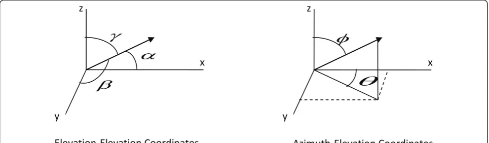
Figure 1 shows an (x,y,z) coordinate axis, with the signal direction of arrival defined in both azimuth-elevation ("az-el”), (θ, ), and elevation-elevation ("el-el”), (a, b) coordinates. As noted in [7], the el-el system allows two
“separate” 1-D angle of arrival measurements from two
Uniform Linear Arrays to be combined. Hence the el-el
format potentially allows an algorithmic complexity reduction by solving separate 1-D problems.
The array response for thenth element in a general
array is most simply written in el-el form,
an(α,β,γ )= exp
−j2π
λ
xn cos(α)+yn cos(β)+zn cos(γ )
(2:1)
where xn, yn, zn define the element position (in
meters) relative to the array axes, a, b, gare the eleva-tion angles relative to the three axes, and lis the sig-nal’s wavelength in meters/cycle. This expression has an intuitively pleasing symmetry: nature should not care
which axis is labeled as x, etc. Only two angles are
needed to determine the direction of arrival, so we can define the third elevation angle from the other two, or,
γ = acos1 - cos2(α)−cos2(β) where acos (x) denotes the inverse cosine. Inserting into (2.1) gives the general array response in el-el coordinates,
an(α,β)= exp
−j2π
λ
xncos(α)+yncos(β)+zn
1−cos2(α)−cos2(β)1/2(2:2) We will consider el-el measurements to be inconsis-tent (meaning no valid direction of arrival can be found) if 1 < cos2(a) + cos2 (b). For consistent angles, we may transform el-el to az-el by noting that:
γ =ϕ
cos(α)= sin(γ )cos(θ) cos(β)= sin(γ )sin(θ)
(2:3)
Direct substitution leads to the general array response in az-el form [2],
an(θ,ϕ)= exp
−j2π
λ
xnsin(ϕ)cos(θ)+ynsin(ϕ)sin(θ)+zncos(ϕ)
(2:4)
Note that the az-el system has no possibility of incon-sistency, but for the special cases of = {0,π} the angle
θ cannot be estimated (hence, the 2-D CRLB does not
exist). Equations 2.2 and 2.4 will be used to create array
T
J
D
E
z
x
y
Elevation-Elevation Coordinates
I
z
x
y
Azimuth-Elevation Coordinates
response vectors for 2-D and 3-D array geometries in following sections. Writing array element coordinates as vectors px, py, pz, the array response vector from the mth source is writtena(θm,m) ora(am,bm)
Angle estimates are mapped to (x,y) position estimates via either,
x y
=Fe αβ
=
zcos(α)1−cos2(α)−cos2(β)−1/2
zcos(β)1−cos2(α)−cos2(β)−1/2
(2:5)
or,
x y
=Fa θϕ
= zcos(θ)tan(ϕ)
zsin(θ)tan(ϕ)
(2:6)
b. Location error ellipses
In a location system, the sources’(x,y) coordinates are of ultimate interest, however, we assume the AOA is esti-mated first, so the system designers can take advantage of modern angle estimation techniques (e.g., MUSIC, ESPRIT, etc.). The estimated angles are then converted to (x,y) estimates, which have a different CRLB. In this section, we show how to draw an error ellipse in the (x, y) plane, containing an area with a specified probability level, corresponding to an (x,y) estimator that achieves the CRLB.
For positive-definite matrix,A, the equationxT Ax= 1 defines an ellipse where the length of each axis from the origin is the inverse square-root of the eigenvalues
of A [14]. Let C=E
θ− ˆθ θ− ˆθH
J−1be the positive-definite error covariance matrix for an estimator that achieves the CRLB. This covariance matrix defines the error“concentration ellipse”with the smallest possi-ble volume (or area, in the 2-D case) [15]. Consider the equation,
c−2θTC−1θ = 1
c−2θTV D−1VHθ = 1
(2:7)
where V, D contain the eigenvectors and eigenvalues of C. Note (2.7) has solutionsθ =cλ1/2i vi, i= 1, 2 cor-responding to the major and minor axes. The values
λ1/2
i are the error standard deviations on the orthogonal
axes, and constant“c“scales the axis lengths proportion-ally. We want to scale the ellipse so that it contains some fraction of the total probability, referred to as a “confidence factor” (CF). As shown in [16], the desired scaling is,
c=−2 ln(1−CF) (2:8)
For example, we can draw an ellipse containing 95% of all estimates, by settingc =2.448.
Note that each point on the error ellipse must satisfy c2 = (Δx)2/l1 + (Δy)
2
/l2, hence we can determine the points on the ellipse (2.7) by stepping through valuesΔx = 0 through cli1/2along one axis, and solving for Δy= ((c2 - (Δx)2/l1)l2)1/2. This creates one quadrant of the ellipse; the rest is produced by symmetry. Finally, the ellipse is centered at the true position, (θ1,θ2).
3. Review of CRLB
a. General principles
The CRLB [2,15,16] gives the lower limit on estimation error among all unbiased estimators. The bound is a useful performance metric, as many practical algorithms have been found to closely approach it at reasonable SNR values [2]. Moreover, the CRLB is a flexible tool that allows modeling many kinds of estimation pro-blems. Most problems involve so-called nuisance vari-ables in addition to the varivari-ables of direct interest. When deriving the bound, nuisance parameters that are known are treated as constants, while those that are
unknown must be included in the parameter vector, θ.
The Fisher matrix is given by
J(θ)=E
d dθ (θ)
d dθ (θ)
H
(3:1)
where Λ(θ) denotes the log-likelihood of the received
vector given the parameters θ, and the expectation is
over the received signal conditioned onθ. The inverse
of the Fisher matrix bounds the achievable error
covar-iance, C ≥J-1 and the diagonal elements ofJ-1 bound
the estimation error of the individual variables.
If a new parameter vector is related to the old one via a change of variables,w=F(θ), then [15],
J−1(w)=F˙TJ−1(θ) F˙, F˙i,j= dwj dθi
(3:2)
gives the new CRLB.
b. Bounds for AOA
Assume a system withNsensors,M sources, andKdata
snapshots. Initially, consider the sources to lie in the plane of the array (1-D angle estimation). The signal vector received at the array for thekth snapshot is,
r(k)=A(θ1)s(k)+n(k) (3:3)
with r Î CNx1, array response matrix A Î CNxM,
source vector s Î CMx1, and where noise vector n Î
covariance σn2IN. Different CRLBs can be derived depending on assumptions regarding the transmitted signals. As shown in [2], three assumptions about the transmitted signalss(k)are commonly used:s(k)is
con-sidered unknown and deterministic (CMA, or
“determi-nistic” bound);s(k)is considered a sample of a complex Gaussian noise process of unknown covariance (UMA, or “stochastic” bound); or finallys(k)can be considered known (most optimistic bound). It seems unlikely that the signal being located would be completely known, hence we will consider only the deterministic and sto-chastic bounds (exceptions are cooperative transmitters acting as beacons, or transmitters using standardized
waveforms having certain features that are known a
priori).
Under 1-D, deterministic assumptions, the
unknown parameter vector is
θθ1,. . .,θM, Re{s(1)}T, Im{s(1)}T,. . ., Re{s(K)}T, Im{s(K)}T
T
consisting of M + 2MK real parameters. The M ×M
upper-left corner of the inverse of the Fisher matrix [2-4] corresponding to the parameters of direct interest (dropping theA(θ)notation for convenience) is,
J−d,11= σ
2 n 2K Re DH
I−AAHA−1AH
D PT −1.(3:4)
Here,
A(θ)=[a(θ1),. . .,a(θM)]
D(θ)= d dθ1
a(θ1),. . ., d
dθM
a(θM)
P=Es sH
(3:5)
The subscript“d,1” indicates this is a deterministic, 1-D bound. Under 1-1-D stochastic assumptions, the
unknown parameter vector is
θθ1,. . .,θM, Re
R1,1
,. . ., ReRN,N
, ReR1,2
ImR1,2
,· · ·, ImRN,N−1
T
consisting ofM+N2unknowns (accounting for
Hermi-tian symmetry), whereRi,j is thei,jth element of the
sig-nal covariance matrix. The M×M upper-left corner of
the inverse of the Fisher matrix [2,4,5] corresponding to the parameters of direct interest is,
J−s,11=
σ2 n 2K Re DH
I−AAHA−1AH
DPAHR−1A PT − 1
R=APAH+σ2
nI
(3:6)
where the subscript “s,1” denotes a 1-D stochastic
bound. The matricesA,D,Pare as in (3.5). The thermal
noise variance may also be considered an‘unknown”but
the bounds (3.4), (3.6) remain unchanged [2].
Next consider a 2-D signal model where it is under-stood that (θ1,θ2) may correspond to either (an,bn), or (θn,n) for allnusers,
r(k)=A(θ1,θ2)s(k)+n(k) (3:7)
At first, it may appear that the new unknowns can
simply be appended to the θ vector and the previous
formulas used. However, the matrix multiplication with
the⊙term in (3.4), (3.6) will no longer be
dimension-ally correct, so a new formula is needed. Deriving com-pact expressions for these formulas turns out to be extremely difficult; however, all the needed results are available in the literature. Under 2-D deterministic assumptions, the unknown parameter vector is
θθ1,1,. . .,θ1,M,θ2,1,. . . θ2,M, Re{s(1)}T, Im{s(1)}T,. . ., Re{s(K)}T, Im{s(K)}T T
consisting of 2M+ 2MKreal parameters. The 2M × 2M
upper-left corner of the inverse of the Fisher matrix [10,11] corresponding to the parameters of direct inter-est is,a
J−1 d,2= σ2 n 2K Re
DHI−AAHA−1
AHD1 21T2⊗PT
−1
D(θ)= dθd 1,1
aθ1,1,θ2,1
,. . .,dθd 1,M
aθ1,M,θ2,M
, d dθ2,1
aθ1,1,θ2,1
,. . ., d dθ2,M
aθ1,M,θ2,M
(3:8)
Finally, under 2-D stochastic assumptions, the
unknown parameter vector is
θθ1,1,. . .,θ1,M,θ2,1,· · ·θ2,M, Re
R1,1
,. . ., ReRN,N
, ReR1,2
ImR1,2
,. . ., ImRN,N−1
T
consisting of 2M +N2unknowns, whereRi,jis thei,jth
element of the signal covariance matrix. The 2M × 2M
upper-left corner of the inverse of the Fisher matrix [8,12] corresponding to the parameters of direct interest is,
J−1 s,2=
σ2
n
2K
ReDHI−AAHA−1
AHD 1 21T2⊗U
−1
U=PAHA P+σ2
nI
−1
AHA P (3:9)
withDas in (3.8). It can be shown thatU =PA HR
-1APT
[4] where R is defined in (3.6) so these UMA
bounds are consistent.
c. 1-D CRLB for the uniform linear array
For the special case of a ULA with a single source, the bounds (3.4) and (3.6) simplify as follows. Assume all the elements are on thex-axis with spacing Δx meters, then,
a= exp
−j2π
λ x[0, 1,. . .,N−1]Tcos(α)
d=−j2π
λ x[0, 1,. . .,N−1]Tsin(α)a PT=P1
(3:10)
Jd,1= 2K P1
σ2 n
Re
−j2π
λxsin(α)aH[0:N−1] I− 1
Ma a H −j2π
λxsin(α)[0:N−1]a
=2K P1 σ2
n
2π
λxsin(α)
2
aH
[0:N−1][0:N−1]a− 1
M
aH [0:N−1]a
2 (3:11)
whereΛx≜diag (x). Then noting,
aH [0:N−1]a=
N−1
n=0
e−jcne+jcnn= N−1
n=0
n=N(N−1) 2
aH
[0:N−1][0:N−1]a= N−1
n=0
e−jcne+jcnn2=
N−1
n=0
n2=N(N−1) (2N−1)
6
Jd,1= 2KP1
σ2 n
2π
λ xsin(α)
21
6
0.5N3+ 2N2−2.5N
J−d,11 6K
SNR2πxsin(α)/λ
2
N3
(3:13)
where c2πx
λ sin(α)and SNR = P1/sn2. Only the
third-order term forNis included in the approximation
(3.13) which agrees exactly with [3]. If we repeat this with the UMA (3.6), the difference lies in the term,
PAHR−1APT=PAH(APA+σI)−1APT which becomes,
P12aH
P1aaH+σn2I
−1
a=P12aHa
P1N+σn2
−1
= P
2 1N P1N+σn2
(3:14)
where the r.h.s. of the first line acknowledges that for the single-user case, steering vectora is an eigenvector ofR. The final expression is,
J−s,11= 6Kσ
2 n
2πx
λ sin(α) 2
N3
P21N P1N+σn2
(3:15)
ForP1Nσn2, the right-hand term in the
denomina-tor converges toP1; hence, the CMA and UMA
expres-sions are asymptotically equal (equal in the limit as
SNR goes to infinity).
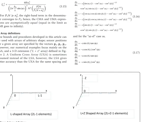
d. Array definitions
The bounds and procedures developed in this article can be used with arrays of arbitrary shape; sensor positions for a given array are specified by the vectorspx,py,pz,. However, our numerical examples focus mainly on the LSA, and a 3-D extension (”L+z“array) defined in Fig-ure 2. A Uniform Cross Array (UXA) is sometimes assumed instead of the LSA, however, the LSA gives better accuracy than the UXA for the same spacing and
number of elements [17]. Practical size constraints may make theL+zarray preferable to the 2LSA.
An array may be decomposed into sub-arrays for “separate”processing. The sensor positions for theqth sub-array are specified by pq, x, pq, y, pq, z. We will assume that the L-shaped array is decomposed into sub-arrays consisting of the x-axis andy-axis elements (the central element is contained in both sub-arrays); theL+ zarray is decomposed into sub-arrays containing the“x andz“and“y andz“ elements, respectively (all elements onz-axis are contained in both sub-arrays). The case of
L+zseparated into three ULAs will not be considered,
as the redundant measurements would need to be
com-bined in somead hocway.
e. Change of variables
To map the 2-D angular CRLBs to bounds on the (x,y)
positions, we use the change of variables (2.5) or (2.6) in (3.2). For the “el-el”case we find the required deriva-tives as,
dxi dαi
=−zsin(αi)
1−cos2(α
i)−cos2(βi) −1/2
+cos2(α
i)sin(αi)1−cos2(αi)−cos2(βi)−
3/2
dxi dβi
=−zcos(αi)cos(βi)sin(βi)1−cos2(αi)−cos2(βi)−3/2
dyi dαi
=−zcos(βi)cos(αi)sin(αi)1−cos2(αi)−cos2(βi)−
3/2
dyi dβi
=−zsin(βi)
1−cos2(α
i)−cos2(βi) −1/2
+cos2(β
i)sin(βi)
1−cos2(α
i)−cos2(βi) −3/2
(3:16)
and for the“az-el”case as,
dxi
dθi
=−zsin(θi)tan(φi)
dxi
dφi
=−zcos(θi)/cos2(φi)
dyi
dθi
=−zcos(θi)tan(φi)
dyi
dφi
=−zsin(θi)/cos2(φi)
(3:17)
0
Z
0
L-1
z
x
y
z
x
y
L-shaped Array (2L-1 elements)
L+Z Shaped Array (2L+Z-1 elements)
The values from (3.16) or (3.17) are inserted into the matrixF˙. Note that for our transformations, all terms dwi/dθjare equal to zero fori≠j, and the matrixF˙ will generally have only two non-zero entries per row or column.
Note that the new CRLB matrix of (3.2) will contain the (x,y) error bounds for all the sources. From this we extract the (2 × 2) matrix for the user of interest, and this becomes the covariance used for drawing concen-tration ellipses described in Section 2b. The joint bound on (x,y) will not depend on the choice of angular coor-dinate system.
4. Separate versus joint bounds
a. Joint bounds
The joint CRLB is computed in a straightforward way, using all the available sensors. Assume that an ordering of the elements is defined, and thatpx, py,pzgive thex,
y, andzcoordinates (in meters) of elements 1 through
N, relative to the array axes.
For the case of el-el coordinates, the mth source has array response vector,
a(αm,βm)= exp
−j2λπpxcos(αm)+pycos(βm)+pz
1−cos2(α m)−cos2(β
m)1/2
(4:1)
The array response matrix is,
A(α,β)=[a(α1,β1),· · ·,a(αM,βM)] (4:2) The derivatives with respect to the estimated para-meters are,
dm,α= d dαm
a(αm,βm)
=j2π
λ
pxsin(αm)−0.5pz
1−cos2(α
m)−cos2(βm) −1/2
sin(2α)a(αm,βm) dm,β= d
dβm a(αm,βm)
=j2π
λ
pysin(βm)−0.5pz
1−cos2(α
m)−cos2(βm)−1/2sin(2β)
a(αm,βm) (4:3)
The derivative matrix is,
D(α,β)=d1,α,· · ·,dM,α,d1,β,· · ·,dM,β
(4:4)
Using (4.2), (4.4), we can compute the deterministic bound (3.8) and the stochastic bound (3.9).
For the case of az-el coordinates,mth source has array response vector,
a(θm,ϕm)= exp
−j2π
λ
pxsin(ϕm)cos(θm)+pysin(ϕm)sin(θm)+pzcos(ϕm)
(4:5)
and the derivatives are,
dm,θ= d dθm
a(θm,φm)
=j2π
λ
pxsin(φm)sin(θm)−pysin(φm)cos(θm)
a(θm,φm) dm,φ= d
dφm a(θm,φm)
=j2π
λ
−pxcos(φm)cos(θm)−pycos(φm)sin(θm)−pzsin(φm)
a(θm,φm)
(4:6)
From these we find A(θ, ), D (θ, ) as before, and compute the deterministic and stochastic bounds.
b. Separate bounds
Assume that the 2-D angle estimation is divided into two separate steps, with each 1-D angle computed from a subset of array elements, or sub-array. The separate bound cannot be lower than the joint bound, as any information about angle 2 that appears in sub-array 1 is ignored, and vice versa. Likewise, any noise correlation due to common elements in the sub-arrays will be ignored. Separate processing is of interest as it may lower the computational complexity of the angle estima-tion algorithm (performing two, 1-D searches may be much easier than performing a single 2-D search). Hard-ware savings are also possible if the radio frequency (RF) chains (i.e., amplifiers, mixers, filters, etc.) associated with the sensors are shared among the sub-arrays, redu-cing the overall cost, size, weight, and power of the
sys-tem. For example, M sensors will only requireM/2 RF
chains if a switching mechanism is used and only one sub-array collects data at a time. As the system spends half the normal observation time collecting samples from each sub-array, and the below bounds would be modified by simply dividing the number of snapshots by 2 (our results do not include this factor of 2). The sepa-rate bound will enable us determine the performance cost of “separate” processing relative to the full (joint) array processing.
To form the separate bound, first we define the ele-ments within each sub-array. Then we find the CRLB under conditions where one angle is being estimated, while the other is unknown. Then, the two resulting Fisher matrices are combined into a single, larger 2M-by-2M matrix. Let pq,x,pq,y,pq,z denote the x,y,z
coordinates of elements in the qth sub-array,q = 1,2.
Assume that the first sub-array will estimate θ1 with
θ2 as an unknown, deterministic nuisance variable,
and likewise the second sub-array estimates θ2 with
θ1 as an unknown. According to CRLB theory, we
must treat both θ1 and θ2 as unknowns to be
esti-mated, but use only the CRLB sub-matrix corre-sponding to the variable being estimated [2,15]. Let
Jt,2(q) denote the Fisher matrix (3.8), (3.9) using only
the elements of the qth sub-array. Define the
“sepa-rate”CRLB as
J−1 t,sep=
W 0M 0M V
, W=J−1
t,2(1)|UL, V=Jt,2−1(2)|LR (4:7)
where t (type) may be either s (stochastic bound) or d
(deterministic bound), and “UL” and “LR” denote
respectively. Note that the block diagonal form of (4.7) results directly from making independent angle esti-mates from the sub-arrays–any beneficial correlation between the angles has been lost. Starting with the joint bound in the deterministic case,
Jd,2=2K
σ2 n
ReDH1A⊥D1PT
ReDH1A⊥D2PT
ReDH2A⊥D1PT
ReDH2A⊥D2PT
(4:8)
whereA⊥I−AAHA−1AHthen using the standard block inversion formulas [18], we can find the UL and LR quantities desired in (4.7) as,
W=σ
2 n
2K
ReD1A⊥D1
PT−ReD1A⊥D2PT
ReD2A⊥D2PT
−1
ReD2A⊥D1PT
−1 (4:9)
V=σ
2 n
2K
ReD2A⊥D2PT
−ReD2A⊥D1PT
ReD1A⊥D1PT
−1
ReD1A⊥D2PT
−1
Breaking the array into non-linear sub-arrays may make it difficult to estimate one angle while the other is unknown, hence complexity may not be reduced. However, if the sub-arrays are linear arrays, then each is only sensitive to a (or,b) and ordinary 1-D estima-tion can be used to reduce the overall complexity. In the case of a linear sub-array, the 2-D CRLB does not exist (i.e., the Fisher matrix is not invertible, as you cannot estimate two angles from a single linear array); so, we use the ordinary 1-D CRLB formulation from each sub-array,
W=J−t,11(1), V=J−t,11(2) (4:10)
c. Separability conditions
Generally, arrays are not“separable”, meaning joint esti-mation will outperform separate estiesti-mation. However, in
some special array geometries the bounds are “
separ-able,”and separate processing is optimal.
Theorem 1 The CRLB for a Uniform Cross Array
(UCA) with a single user is separable.
This result is stated in [17] for the deterministic case
without proof. For the UCA with 2L-1 elements (L
assumed odd), the array position vectors are,
px
vx,01×(L−1)T,vx=[−NUCA,. . .,−1, 0, 1,. . .,NUCA],
NUCA=
L−1 2 py
01×L,vy
T
,vy=[−NUCA,. . .,−1, 1,. . .,NUCA]
(4:11)
For the single user case,
a(α,β)= exp
−j2π
λx
pxcos(α)+pycos(β) ∈C2L−1×1
A⊥=I−aaHa−1aH=I− 1
2L−1a a
H
dα=j2π
λ xpxsin(α)a(α,β)=j
2π
λxsin(α) pxa(α,β) dβ=j2π
λ xpysin(β)a(α,β)=j
2π
λ xsin(β) pya(α,β)
(4:12)
where Λx ≜ diag (x) is a diagonal matrix. Inserting into (4.8), we want to prove that the resulting matrix has the form (4.7). Beginning with the upper-right term,
DH 1A⊥D2=aHpx
I− 1
2L−1a a
H
pya=aHpxpya− 1
2L−1
aH
pxa aHpya ?
=0
= 0−aH pxa aHpya
aH pxa =
2L−1 i=1
ej f(i)e−j f(i)p
x(i)= sum
px
=sum(vx)= 0
(4:13)
Where f(i) is a real-valued function corresponding to the exponent of the array response vector, the fact that
Λpx Λpy = 0, and that the sum over vx is zero by
inspection. Now turning to the upper-left term, and definingaaT
1,aT2
T ,
DH1A⊥D1=
j2πx
λ cosα 2
aH1vx
IL− 1 2L−1a1a
H 1
vxa1(4:14)
By inspection, this term is equal to the 1-D bound J1,d (1) except for the scale factor 2L-1. However, for the special case under consideration, this term is zero becauseaH1vxa1= sum(vx)= 0.
Likewise, we may show that the lower-left term is zero and the lower-right term isJ1,d(2) which completes the proof in the deterministic case. However, as only prop-erties ofDHA⊥Dwere used, the result extends immedi-ately to the stochastic case as well.
Theorem 2 The CRLB for an L-shaped Array (LSA)
with a single user is not separable.
For the LSA with 2L-1 elements, the element position vectors are
px
ux,01×(L−1)T, ux=[0, 1,· · ·,L−1] py01×L,uy
T
, uy=[1,· · ·,L−1]
Examining the term DH1A⊥D2, as in the upper-right term of (4.8),
2πdλ 2
cosαcosβaH
x
I− 1
2L−1a a
H
ya
=
2πλd
2
cosαcosβ
− 1
2L−1 a
H
xa aHya
aH
xa
=aH 1,aH2
diag(ux)0
0 0
a1 a2
=aH
1diag(ux)a1= sum(ux)= 0 Likewise,aH
ya
= 0
An intuitive explanation for Theorem 2 is to note that the LSA is able to make measurements over a “long baseline” pair–the pair of sensors at the tips of the two arms. There are no two elements within a sub-array having as large a spacing as this, giving an advantage to the joint processing for LSA. By contrast, the tip-to-tip distance in the UCA does not exceed the largest spacing found in a sub-array, and there is no such advantage.
Theorem 3 The 2-D CRLB is non-increasing in the
number of sensors (regardless of their positions).
This is an extension to the 2-D case of a proof in [3]
for the deterministic case. Consider a system with N
sensors,AÎCN×M,DÎCN×2M, and the Fisher matrix,
J= σ 2
n
2K
ReDH
αA⊥DαPTReDH
βA⊥DαPT ReDH
αA⊥DβPTReDH
βA⊥DβPT
(4:15)
Adding an extra sensor,
¯ A= A
uT
, D¯ =D¯αD¯β, D¯α= Dα
vT
α
(4:16)
The new system (with over-bar notation) has Fisher matrix,
¯ J= σ
2 n 2K ⎡ ⎣Re ¯ DHαA¯⊥D¯α
PTReD¯H
βA¯⊥D¯α
PT
Re
¯ DHαA¯⊥D¯β
PTReD¯H
βA¯⊥D¯β
PT
⎤ ⎦ (4:17)
Note that,
¯
A⊥IN+1− ¯A
¯
AHA¯−1A¯H
= IN0
0T1
− uAT AHA+u∗uT
−1
AHu∗ (4:18)
AHA+u∗uT−1 =AHA−1
−
AHA−1
uTu∗AHA−1 1 +uTAHA−1
u∗
=AHA−1
−(4:19)
Focusing on the upper-left term of (4.17),
¯
DHαA¯⊥D¯α=DH αv∗α
IN0
0T1
− uAT AHA −1
− AHu∗ Dα vT α
(4:20)
Following the somewhat involved algebra of [3, App. F] this can be simplified to,
¯
DHαA¯⊥D¯α=DH
αA⊥Dα+εαεαH, εα=v ∗
α−DHαAAHA−1u∗
1 +uTAHA−1
u∗ (4:21)
Likewise, for the three remaining terms in (4.17) we can show,
¯
DHβA¯⊥D¯α=DHβA⊥Dα+εβεHα
¯
DHαA¯⊥D¯β=DHαA⊥Dβ+εαεHβ
¯
DHβA¯⊥D¯β=DHβA⊥Dβ+εβεHβ
(4:22)
The Fisher matrix is now,
¯
J= Re D
H
αA⊥DαDHαA⊥Dβ
DH
βA⊥DαDH
βA⊥Dβ
+ εεα β εα εβ H
PPTTPPTT
=J+ Re εεα
β
εα
εβ
H
PPTTPPTT
J+ ReE ¯P
(4:23)
The matrixP¯ is easily found to be positive semi-defi-nite (psd) as follows. SincePTis a covariance matrix we
can write it in terms of eigenvectors and eigenvalues as
PT
=VDVH. The matrixP¯ has 2M eigenvectors, which
by inspection are ¯v=vT
i,vTi
T
,vT
i,−vTi
T
, and the eigenva-lues areλ¯i= 2λiandλ¯i= 0(with multiplicity M). Hence, for PT ≥ 0, it follows thatP¯ ≥0. Next, it follows from
the Schur Product Theorem that E ¯P≥0since the
individual matrices are psd. Then, X ≥0 ⇒ Re {X} ≥ 0
for X Hermitian. So, we can state, ¯J≥J, and¯J−1≤J−1,
which completes the proof for the deterministic case. To extend the result to the stochastic case, it is only
necessary to prove that U ≥ 0, which follows directly
from the factorizationU= (R-1/2AHP)H(R-1/2AHP).
5. Numerical results
Unless otherwise stated, our numerical results assume a
LSA of 11 elements (L= 6), spaced at half-wavelength
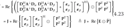
and the CMA is used. The instantaneous SNR = 10 dB, 15 snapshots are used, and we set CF = 0.95. The array height is either 1500 or 3000 ft; there is no fading or multipath. Figure 3 compares error ellipses for separate processing at two heights and two locations. In Figure 3a the source is almost under the array, at (0.25, 0.25) km. The confidence contours are nearly circular, and notice the position error is smaller at lower height. On the other hand, Figure 3b shows a more distant source at (0.75, 0.75) km. Now the position error is smaller at the greater height. This demonstrates a basic trade-off for our location geometry: distant sources require greater array height. Intuitively, for a distant source, lower height increases the error two ways: the source is increasingly off-boresight which reduces the effective aperture size, i.e., the sin(a) dependence seen in (3.13), and simultaneously, the error contour expands like a
“lengthening shadow” when projected to the ground
plane.
processing. As seen, joint processing seems particularly beneficial when multiple sources are present. We repeated Figure 4a,b under the UMA, and the results appeared equivalent (not shown).
In Figure 5, the interferer is moved to the location (0.5, -1.95). Note that a linear array is subject to an “ambiguity cone": identical array responses are created by sources rotated around the array axis. Here, an origi-nal source at (0.25, 0.75) and another source anywhere along the line c(0.25,-0.75) creates the same response. The interferer in Figure 5 is nearly on this line (c= 2) and the related A(θ1, θ2) matrix is ill-conditioned as both sources have nearly the same response vector. As seen, the separate approach produces a very large
ellipse. However, the joint approaches give excellent error performance, as in the larger space (with dimen-sion 2L- 1) the A(θ1,θ2) matrix is not ill-conditioned.
In Figure 6 we compare the LSA with theL +z array
having two additional elements on the z-axis (z = 2). In Figure 6a, a single source is present. The LSA is shown
with separate and joint processing as before. The L+z
with separate processing shows only a very small gain relative to LSA; however, joint processing shows a strong improvement. In Figure 6b, a single interferer is present, and some additional improvement between LSA
and L+z with separate processing is observed. Again,
large gains are seen obtained for L +z over LSA with
joint processing. The “lengthening shadow” effect can be
significantly reduced by joint processing of the L+ z
array; it is reduced by about 50%. A
B
Figure 3Separate processing at two heights (1500 and 3000 ft).(a)Source at (0.25, 0.25) km.(b)Source at (0.75, 0.75) km.
A
B
In Figure 7 we repeat the comparison of LSA vs. L+
z, but with constant number of elements, and a single
interferer. Take LSA, joint processing withL= 5 (9 ele-ments in total) as a baseline. Consider adding two addi-tional elements, either the LSA with L= 6, or theL+z
with L= 5 andz = 2, each having 11 elements in total.
As seen, for this geometry, theL+zis much preferred;
theL+z ellipse has the same width as theL= 5
base-line, but much reduced length.
6. Conclusions
Two-dimensional angle-of-arrival estimation can be used to locate ground sources on the ground plane from a single array. The 2-D CRLB must be used to bound the performance, and we were able to find the needed bounds in the literature for both the Conditional Model Assumption (CMA) and the Unconditional Model Assumption (UMA). Some location systems may use
suboptimal “separate” estimation of the two spatial
angles, and this required us to modify the bounds. Our numerical examples show that joint processing has con-siderable advantage when interferers are present, parti-cularly when an interferer lies near the“ambiguity cone” of the source. We also showed that adding additional elements along the z-axis can be very beneficial for dis-tant sources when joint processing is used.
Endnotes a
[10,11] give the second term inside the braces as PT⊗121T2 and giveD in a “parameters-first” ordering. Elementary permutation matrices can be used to reorder theirDto be consistent with (3.9) in“users-first” order-ing, which changes (3.8) to the form shown. Users-first ordering is preferred to analyze the“separate”bounds. Figure 5L-array with a single interferer.
A
B
Figure 6L+zarray.(a)LSA vs.L+zwith no interference.(b)LSA vs.L+zwith one interferer.
Abbreviations
AOA: Angle-of-arrival; CMA: Conditional Model Assumption; CRLB: Cramer-Rao lower bound; CF: confidence factor; LSA: L-shaped array; 1-D: one-dimensional; psd: positive semi-definite; RF: radio frequency; 2-D: two-dimensional; 2LSA: two L-shaped array; UXA: Uniform Cross Array; UMA: Unconditional Model Assumption.
Competing interests
The author declares that they have no competing interests.
Received: 30 November 2010 Accepted: 13 May 2011 Published: 13 May 2011
References
1. H Krim, M Viberg, Two Decades of Array Signal Processing Research. IEEE Signal Processing Magazine. (1996)
2. HL van Trees,Optimum Array Processing: Detection, Estimation, and Modulation Theory, Part IV. (Wiley-Interscience, Hoboken, NJ, 2002) 3. P Stoica, A Nehorai, MUSIC, Maximum-Likelihood, and Cramer-Rao bound.
IEEE Transactions on Acoustics, Speech, and Signal Processing.37(5) (1989) 4. P Stoica, A Nehorai, Performance study of conditional and unconditional
direction-of-arrival estimation. IEEE Transactions on Acoustics, Speech, and Signal Processing.38(10) (1990)
5. P Stoica, E Larsson, A Gershman, The Stochastic CRB for array processing: a textbook derivation. IEEE Signal Processing Letters.8(5) (2001)
6. N Tayem, H Kwon, L-shape 2-dimensional arrival angle estimation with propagator method. IEEE Transactions in Antennas and Propagation.53(5) (2005)
7. S Kikuchi, H Tsuji, A Sano, Pair-matching method for estimating 2-D angle of arrival with a cross-correlation matrix. IEEE Antennas and Wireless Propagation Letters.5(2006)
8. T Xia, Y Zheng, Q Wan, X Wang, Decoupled estimation of 2-D angles of arrival using two parallel uniform linear arrays. IEEE Transactions on Antennas and Propagation.55(9) (2007)
9. M Li, L Gan, P Wei, Improvement of 2-D direction finding algorithm based on two L-shape arrays. ICSP. (2008)
10. SZ Yau, Y Bresler, A compact Cramer-Rao bound expression for parametric estimation of superimposed signals. IEEE Transactions on Signal Processing. 40(5) (1992)
11. ST Smith, Statistical resolution limits and the complexified Cramer-Rao bound. IEEE Transactions on Signal Processing.53(5) (2005) 12. A Nehorai, E Paldi, Vector-sensor array processing for electromagnetic
source localization. IEEE Transactions on Signal Processing.42(2) (1994) 13. DT Vu, A Renaux, R Boyer, S Marcos, Performance analysis of 2D and 3D
antenna arrays for source localization. 18th European Signal Processing Conference, EUSIPCO-2010
14. G Strang,Linear Algebra and its Applications. (Harcourt, Brace, Jovanovich, San Diego, CA, 1988)
15. LL Scharf,Statistical Signal Processing. (Addison-Wesley Publishing, New York, 1991)
16. HL van Trees,Detection, Estimation, and Modulation Theory: Part I. (Wiley, New York, 1968)
17. Y Hua, T Sarkar, D Weiner, An L-shaped array for estimating 2-D directions of wave arrival. IEEE Transactions on Antennas and Propagation.39(2) (1991)
18. T Kailath,Linear Systems. (Prentice-Hall Inc, Englewood Cliffs, NJ, 1980)
doi:10.1186/1687-6180-2011-5
Cite this article as:Mailaender:Bounds for 2-D angle-of-arrival estimation with separate and joint processing.EURASIP Journal on Advances in Signal Processing20112011:5.
Submit your manuscript to a
journal and benefi t from:
7Convenient online submission
7Rigorous peer review
7Immediate publication on acceptance
7Open access: articles freely available online
7High visibility within the fi eld
7Retaining the copyright to your article