Fast Fourier Orthogonalization
Léo Ducas
∗ CWI, Cryptology Group Amsterdam, The NetherlandsThomas Prest
†Thales Communications & Security Gennevilliers, France
ABSTRACT
The classical fast Fourier transform (FFT) allows to compute in quasi-linear time the product of two polynomials, in the
circular convolution ringR[x]/(xd−1) — a task that naively requires quadratic time. Equivalently, it allows to accelerate matrix-vector products when the matrix iscirculant.
In this work, we discover that the ideas of the FFT can be applied to speed up the orthogonalization process of matrices with circulant blocks of sized×d. We show that, whendis composite, it is possible to proceed to the orthogonalization in an inductive way —up to an appropriate re-indexation of rows and columns. This leads to a structured Gram-Schmidt decomposition. In turn, this structured Gram-Schmidt de-composition accelerates a cornerstone lattice algorithm: the nearest plane algorithm. The complexity of both algorithms may be brought down to Θ(dlogd).
Our results easily extend tocyclotomic rings, and can be adapted to Gaussian samplers. This finds applications in lattice-based cryptography, improving the performances of trapdoor functions.
Keywords. Fast Fourier transform, Gram-Schmidt or-thogonalization, nearest plane algorithm, lattice algorithms, lattice trapdoor functions.
1.
INTRODUCTION
When operations involving linear algebra are to be per-formed over structured matrices, a natural problem is to accelerate them by exploiting the structure. The most classi-cal example is the fast Fourier transform [2, 8], which allows to perform matrix-vector multiplication in quasilinear time
∗This work has been supported by a grant from CWI from budget
for public-private-partnerships and in part by a grant from NXP Semiconductors. Part of this work was also supported by an NWO Free Competition Grant.
†
Part of this work was done when the author was at the ´Ecole Normale Sup´erieure, Paris. This work was partially funded by the European Union H2020 SAFEcrypto project (grant no. 644729).
Full version of the article to appear at the 41st International Symposium on Symbolic and Algebraic Computation (ISSAC 2016).
when the matrix is circulant. This is achieved by exploiting the isomorphism between the ring ofd×dcirculant matrices and thecircular convolution ringRd=R[x]/(xd−1).
A widely studied and more involved question is matrix decomposition [20] for structured matrices, in particular Gram-Schmidt orthgonalization (GSO). In this work, we are interested in the GSO ofcirculant matrices, and more gener-ally of matrices with circulant blocks. Our main motivation is to accelerate lattice algorithms for lattices that admit a basis with circulant blocks. This use case allows a helpful extra degree of freedom: one may permute rows and columns of the lattice basis since this leaves the generated lattice unchanged —up to an isometry.
As we will show, a proper re-indexation of these matri-ces highlights an inductive structure, with a fast Fourier flavor. This leads to accelerations of the orthogonalization process —and of the related nearest plane algorithm— down to quasilinear time and space.
The Nearest Plane Algorithm, Lattices and
Cryptography
The nearest plane algorithm [1] is a central algorithm over lattices. It allows, after precomputation of the GSO and using a quadratic number of real operations, to find a rel-atively close point in a lattice to an arbitrary target. It is a core subroutine of LLL [13], and can be used for error correction over analogical noisy channels. It has also found applications in lattice-based cryptography as a decryption al-gorithm, and a randomized variant (called discrete Gaussian sampling) [11, 5] provides secure trapdoor functions based on lattice problems. This leads to cryptosystems (attribute-based encryption) with fine-grained access control, as [18, 6] to name a few.
Given a basisBof a latticeL⊂Rdand a target vectorc, the nearest plane algorithm finds a lattice point somewhat close to c. The result belongs to a fundamental domain centered inc, whose shape is the cuboid defined by ˜B, the GSO ofB(see Figure 1). This algorithm performs Θ(d2) real
operations. The GSO itself is required as a precomputation.
Structured lattices in cryptography.
This is sometimes referred as lattice-based cryptography in thering setting. Technically, the chosen rings typically are
cyclotomic rings, but those are closely related to the convo-lution ringsdiscussed so far. The core of this optimization is the fast Fourier transform (FFT) [2, 4, 8, 19] allowing fast multiplication of polynomials. But this improvement did not apply in the case of the nearest plane algorithm or its randomized variant [11, 5]: na¨ıve GSO do not take the algebraic structure into account.
One possible work-around [9, 22] consist of using the round-off algorithm [1] instead of the nearest-plane algorithm. How-ever, this simpler algorithm outputs further vectors, both in the average and worst cases, weakening those cryptosystems.
c c
Round-off Nearest plane
Figure 1: Round-off and nearest plane algorithms, and their associated fundamental domains.
Our contribution
In this work, we discover new algorithms, obtained by cross-ing Cooley-Tukey’s [2] fast Fourier transform algorithm to-gether with the orthogonalization and nearest plane algo-rithms (not exactly the GSO, but the closely related LDL? de-composition). Precisely, we show that, up to a re-indexation of rows and columns, the orthogonalization of matrices com-posed ofd×d-circulant blocks can be done in time Θ(dlogd) when the prime factors ofdare bounded. Our algorithm pro-duces the LDL? decomposition in a special compact format, requiring Θ(dlogd) complex numbers to represent.
From this compact representation, the nearest plane algo-rithm can also be performed using Θ(dlogd) real operations.1 As a demonstration of the simplicity of our algorithms, we propose an implementation in python for d×d-circulant matrices, whendis a power of 2.
Computational model and Parallelism.
Our algorithms and their complexity are described for Random Access Machines with unitary arithmetic operations onreal numbers, i.e. we do not study the issue related to floating-point approximations and numerical stability.
Regarding parallelism, we note that our Fast-Fourier LDL? algorithm is almost fully parallelizable: viewed as an arith-metic circuit on real numbers, it has depthO(log(n)) and widthO(n). This is unfortunately not the case of the Nearest Plane algorithm nor our Fast-Fourier variant, for which the
nrounding steps are inherently sequential.
Techniques.
At the core of our techniques is the realization that repre-senting elements of the convolution ringRd=R[x]/(xd−1) as circulant matrices is not the appropriate choice. To allow an induction similar to Cooley-Tukey’s FFT, our representation
1If the numbern×mofd×dcirculant blocks is not constant,
they contribute a factorO(n3) to the runtime of the fast-Fourier LDL?algorithm,O(n2) to its output size, andO(n2)
to the run-time of the fast-Fourier nearest plane algorithm.
must follow thetower of ringsR⊂ Rd1⊂ · · · ⊂ Rdi−1 ⊂ Rd, for some chain of divisors 1|d1|. . .|di−1|d.
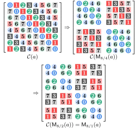
Such a representation is obtained by applying the (mixed-radix) digit-reversal order to the indexation of the rows and column of the circulant blocks, as pictured in Figure 2.
We show that this alternative indexation allows to repre-sent the matrixLof the GSO in a factorized form: a product of Θ(logd) (sparse) structured matrices, each of which can be stored in spaceO(d). An example is given in Figure 3.
Once this hidden structure is unveiled (Theorem 1), the al-gorithmic implications follow quite naturally: one first easily derive an algorithm in timeO(nlog2n) —matching previous and more general results [21]— but noting that the splitting step may be performed directly in the Fourier domain al-lows us to save another lognfactor. For easier algorithmic manipulations, the factorization ofLis represented using a tree.
0 1 2 3 4 5 6 7 7 0 1 2 3 4 5 6 6 7 0 1 2 3 4 5 5 6 7 0 1 2 3 4 4 5 6 7 0 1 2 3 3 4 5 6 7 0 1 2 2 3 4 5 6 7 0 1 1 2 3 4 5 6 7 0
⇒
0 2 4 6 1 3 5 7
6 0 2 4 7 1 3 5 4 6 0 2 5 7 1 3
2 4 6 0 3 5 7 1
7 1 3 5 0 2 4 6 5 7 1 3 6 0 2 4
3 5 7 1 4 6 0 2
1 3 5 7 2 4 6 0
C(a) C(M8/4(a))
⇒
0 4 2 6 1 5 3 7
4 0 6 2 5 1 7 3
6 2 0 4 7 3 1 5
2 6 4 0 3 7 5 1
7 3 1 5 0 4 2 6
3 7 5 1 4 0 6 2
5 1 7 3 6 2 0 4
1 5 3 7 2 6 4 0
C(M8/2(a)) =M8/1(a)
Figure 2: Re-indexing the transformation matrix of
f∈ R87→f x(a= 0 +x+ 2x2+· · ·+ 7x7∈ R8) .
L= 1 1 1 1 a b c d 1 b a d c 1
d c a b 1
c d b a 1
· 1 1 e f 1 f e 1
1 1 g h 1 h g 1
· 1 i 1 1 j 1 1 k 1 1 l 1 L: a b c d g h l k e f j i
Related Works.
There exist many works related to the orthogonalization of structured bases. For Toeplitz matrices, Sweet [23] intro-duced an algorithm faster than the naive orthogonalization by a linear factor. Gragg [7] has shown that for Krylov bases – which are bases of the form{b, r(b), ..., rd−1(b)} –, the Levinson recursion [14, 3] allows, whenr is an isometric operator, to perform orthogonalization in time Θ(d2) instead
of Θ(d3).
There also exists superfast (running timeO(nlog2n)) algo-rithms for the orthogonalization of Toeplitz-like matrices, for example by Olshevsky and Pan [21], and those are already based on a structure-preserving induction. In this light, one may interpret our result as a Fourier-compatible version of these superfast algorithms.
The question of improving the nearest-plane algorithm for structured matrices seems less studied. As far as we know, the state of the art consist of a single result [17], applying the Levinson recursion [14] to reduce by a linear factor itsspace
complexity. Alternatively, a work-around of lesser quality was proposed for the NTRU signature scheme [9, 22].
Outline.
Section 2 introduces the mathematical tools that we will use through this paper. Section 3 presents our main result, namely the existence of a compact, factorized representation for the GSO and LDL? decomposition, and gives a fast Fourier flavored algorithm for computing it in this form. This compact LDL? decomposition is further exploited in Section 4, which presents a nearest plane algorithm that also has an FFT flavor. Appendix A extends all our results from convolution rings to cyclotomic rings, by reducing the latters to the formers. Appendix B demonstrates the practical feasibility of our algorithms by presenting a rather succinct
python implementations of them in the case whered is a power of two. The full prototype implementation inpython
—forda power of 2— is also available online.2
2.
PRELIMINARIES
For any ringR,R[x] will denote the ring of univariate poly-nomials overR. Scalars (which includes elements ofR) will usually be noted in plain letters (such asa, b), vectors will be noted in bold letters (such asa,b) and matrices will be noted in capital bold letters (such asA,B). Vectors are mostly in row notation, and as a consequence vector-matrix products are done in this order unless stated otherwise. (a1, . . . , an) de-notes the row vector formed of theai’s, whereas [a1, . . . ,an]
denotes the matrix whose rows are theai’s. Ndenotes the set of non-negative integers, and N∗ the set N\{0}. For
i, j∈Z,Ji, jKwill denote the set{i, i+ 1, . . . , j−1, j}.
2.1
The Convolution Ring
R
dDefinition 1. For anyd ∈ N∗, let Rd denote the ring R[x]/(xd−1), also known as circular convolution ring, or
simply convolution ring.
Whendis highly composite, elementary operations inRd can be performed in time Θ(dlogd) using the fast Fourier transform [2].
2
https://github.com/lducas/ffo.py
We equip the ringRdwith a conjugation operation as well as an inner product, making it an Hermitian inner product space. The definitions that we give also encompass other types of rings that will be used in Appendix A.
Definition 2. Leth∈R[x]be a monic polynomial with
distinct roots overC,R=∆R[x]/(h(x))anda, bbe arbitrary
elements ofR.
• We notea?and call (Hermitian) adjoint ofathe unique element ofRsuch that for any rootζofh,a?(ζ) =a(ζ), where·is the usual complex conjugation overC.
• The inner product overRisha, bi=∆P
h(ζ)=0a(ζ)·b(ζ),
and the associated norm iskak=∆pha, ai.
In the particular case of convolution rings, one can check that ifa(x) =Pd−1
i=0aixi∈ Rd, then
a?(x) =a(1/x) mod (xd−1) =a0+ d−1
X
i=1 aix
d−i
.
The (Hermitian) adjointB? of a matrixB∈ Rn×m is the transpose of the coefficient-wise adjoint ofB.
While the inner producth·,·i(resp. the associated norm k · k) is not to be mistaken with the canonical coefficient-wise dot producth·,·i2 (resp. the associated norm k · k2), they
are closely related. One can easily check that for anyf = P
i∈Zdfixi ∈ Rd, the vector (f(ζ)){ζd=1} can be obtained from the coefficient vector (fi)06i<dby multiplying it by the Vandermonde matrixVd= (ζdij)06i,j<d, where ζd denotes an arbitraryd-th primitive root of unity. The matrixVd satisfies VdV?d =d·Id and as an immediate consequence: hf, gi=d· hf, gi2.
Definition 3. Letm>nandB={b1, . . . ,bn} ∈ Rn×m. We say thatBis full-rank (or is a basis) if for any linear com-binationP
16i6naibi withai∈ R, we have the equivalence (P
iaibi=0)⇐⇒(∀i, ai= 0).
We note that sinceRis generally not an integral domain, a set formed of a single nonzero vector is not necessarily full-rank. In the rest of the paper, a basis will either denote a set of independent vectors {b1, . . .bn} ∈(Rm
)n, or the full-rank matrixB∈ Rn×mwhose rows are thebi’s.
2.2
The GSO and LDL
?Decomposition
In this section,R=R[x]/(h(x)) as in Definition 2. We first recall a few standard definitions. A matrixL∈ Rn×n is unit lower triangular if it is lower triangular and has only 1’s on its diagonal.We say that a self-adjoint matrixG∈ Rn×n is full-rank Gram (or FRG) if there existm>nand a full-rank matrix B∈ Rn×m
such thatG=BB?. This generalizes the notion of positive definiteness for symmetric real matrices.
We now recall the GSO and LDL? decomposition. The GSO decomposes any full-rank matrix as the product of a unit lower triangular matrix and an orthogonal matrix.
Proposition 1. LetB∈ Rn×m
be a full-rank matrix. B
can be uniquely decomposed as
B=L·B˜, (1)
WhenRis replaced byRor a number field, Proposition 1 is standard. In our case, a proof can be found in Appendix C. The LDL?decomposition writes any positive definite ma-trix as a product LDL?, where L ∈ Rn×n
is unit lower triangular with 1’s on the diagonal, andD∈ Rn×n
is diago-nal. It is related to the GSO as for a basisB, there exists a unique GSOB=L·B˜ and for an FRG matrixG, there ex-ists a unique LDL?decompositionG=LDL?. IfG=BB?, thenG=L·( ˜BB˜?)·L?is a valid LDL?decomposition of G. As both decompositions are unique, the matricesLin both cases are actually the same. In a nutshell:
L·B˜ is the GSO ofB
⇔ L·( ˜BB˜?)·L?is the LDL?decomposition of (BB?).
Algorithm 1LDL?R(G)
Require: A full-rank Gram matrixG= (Gij)∈ Rn×n. Ensure: The decomposition G=LDL? overR, whereL
is unit lower triangular andDis diagonal. 1: L,D←0n×n
2: forifrom 1 tondo 3: Lii←1
4: Di←Gii−Pj<iLijL?ijDj 5: forjfrom 1 toi−1do 6: Lij←D1
j
Gij−Pk<jLikL?jkDk
7: end for 8: end for
9: return ((Lij),Diag(Di))
Algorithm 1 computes the LDL?decomposition. WhenR is replaced byR, the decomposition is noted LDL? rather than LDL?and it is well-known that it terminates without encountering divisions by 0 . In our case, we prove that it terminates correctly in Appendix C.
2.3
Babai’s Nearest Plane Algorithm
The nearest plane algorithm allows to find a lattice close to an arbitrary target in the ambient vector space. Precisely, it ensures that the difference between the target and the output lies in the fundamental parallelepiped spanned by the GSO ˜Bof a given lattice basisB, as depicted on Figure 1.
Definition 4. LetB={b1, . . . ,bn}be a real basis. We
call fundamental parallelepiped generated byBand noteP(B)
the set P
16j6n
−1
2, 1 2
bj= −1
2, 1 2
n ·B.
Algorithm 2NPR(t,L)
Require: The decompositionB=L·B˜ of B ∈Rn×m, a vectort∈Rn
Ensure: A vectorz∈Znsuch that (t−z)B∈ P( ˜B) 1: z←0
2: forj=n, . . . ,1do
3: ¯tj←tj+Pi>j(ti−zi)Lij 4: zj← b¯tje
5: end for 6: return z
Proposition 2 (From [1, 13]). Algorithm 2 outputs an integer vectorz(zB∈ L(B)) such that(t−z)B∈ P( ˜B).
2.4
Coefficient Vectors and Circulant
Matri-ces
Definition 5. We define linear mapsc:Rm d →R
dm
and
C:Rn×md →Rdn×dm as follows. For anya=Pi∈Zdaixi∈ Rdwhere eachai∈R:
1. The coefficient vector ofaisc(a) = (a0, . . . , ad−1).
2. The circulant matrix ofais
C(a)=∆
a0 a1 · · · ad−1 ad−1 a0 · · · ad−2
. .. . .. . .. . ..
a1 a2 . . . a0
=
c(a)
c(xa)
. . .
c(xd−1a)
∈Rd×d.
3. candCgeneralize to vectors and matrices in a coefficient-wise manner.
Proposition 3. The mapscand C satisfy the following
properties:
1. C is an injective algebra morphism. In particular,
C(a)C(b) =C(ab). 2. c(a)C(b) =c(ab). 3. C(a)?=C(a?).
Proposition 3, item 2 illustrates the following fact: the mapscandCare complementary. Indeed, if we consider the ordered R-basisB= {1, x, . . . , xd−1} of Rd, then cis the map that writes any a ∈ Rd as its unique decomposition according toB. Similarly, for the same basis,C(a) is the transformation matrix of the injective mapf ∈ Rd7→f a. This is the intrinsic reason that makes Proposition 3, item 2 true.
In Section 2.5, we will define mapsV,M which will be complementary in the same way asc,C are.
2.5
Linearization Operators
In this section, we introduce two partial linearization oper-ators, a vectorial one denoted byVd/d0 (orV), and a matricial one denoted byMd/d0 (orM).
They are very similar toc,C. Indeed, for anyd0|d and
a∈ Rd,Vd/d0(a) will writeaas a vector of theRd0-module Rd/dd0 0, and Md/d0(a) will be the matrix associated to the injective mapf∈ Rd7→f a. They are in fact generalizations of the maps from Section 2.4:
1. Rdmay not only be seen as ad-dimensionalR-vector space, but also as ad/d0-dimensionalRd0-module for anyd0|d.
2. When writingRd as ad-dimensionalR-vector space, we will not use{1, x, . . . , xd−1}as our canonical basis,
but a permutation of this basis
Definition 6. Let d∈N∗ be a product ofh (not
neces-sarily distinct) primes. Letgpd(d)denote the greatest proper divisor of d. When clear from context, we also note h the number of prime divisors of d (counted with multiplicity),
dh
∆
=dand fori∈J1, hK,di−1gpd(di)andki ∆
=di/di−1, so
that1 =d0|d1|. . .|dh=dandQj6ikj=di.
Definition 7. Letd, d0∈N∗such thatd0 is in the tower
of proper divisors ofd, and letk=d/d0. We denote byxthe indeterminate of the polynomial ringRd=R[x]/(xd−1)and
byy =xk the indeterminate ofR
d0 =R[y]/(yd 0
−1). We define the partial linearizationVd/d0:Rmd → Rkmd0 recursively
as follows:
1. Ford=d0= 1,Vd/d0 is the identity.
2. For d0 = gpd(d) and a single element a ∈ Rd, let
a=P
i∈Zkx i
ai(y)whereai∈ Rd0 for each i. Then
Vd/d0(a)∆= (a0, . . . , ak−1).
In other words,Vd/d0(a)∈ Rkd0 is the row vector whose
coefficients are the(ai)i∈Zk.
3. For a vectorv∈ Rm
d,Vd/d0(v)∈ Rkmd0 is the
component-wise applications of Vd/d0.
4. Ford00|d0|d and any vectorv∈ Rm d, Vd/d00(v)=∆Vd0/d00◦Vd/d0(v)∈ R(d/d
00)m d00 .
Whendis clear from context, we simply noteVd/d0 =V/d0.
Interpretation.
In practice, an elementa ∈ Rd is represented by a vector ofd real elements corresponding to thedcoefficients of a. In this context, the operatorVsimply permutes coefficients. As highlighted by Figure 4, whend= 2his a power of two, Vd/1 permutes the coefficients according to the bit-reversal
order3, which appears in the radix-2 fast Fourier transform (FFT). More generally, one can show that for an arbitraryd, Vd/1permutes the coefficient according to the general
mixed-radix digit reversal order, which appears in the mixed-mixed-radix Cooley-Tukey FFT [2].
0 1 2 3 4 5 6 7 ⇒ 0 2 4 6 1 3 5 7
c(a) c(V/4(a))
⇒ 0 4 2 6 1 5 3 7
c(V/2(a)) =V/1(a)
Figure 4: Partial vectorial linearizations.
We now move to the matrix representationMcompatible withV.
Definition 8. Following the notations of Definition 7, we define the operatorMd/d0 :Rn×m
d → R
kn×km
d0 as follows:
1. Ford=d0= 1,Md/d0 is the identity.
2. For d0 = gpd(d), k=d/d0 and a single element a= P
i∈Zkx ia
i(y) where each ai ∈ Rd0, Md/d0(a) is the
following matrix of∈ Rk×k d0 :
a0 a1 · · · ak−1 yak−1 a0 · · · ak−2
. .. . .. . .. . ..
ya1 ya2 . . . a0
=
Vd/d0(a) Vd/d0(xka)
. . .
Vd/d0(x(d 0−1)k
a)
.
In particular, ifd is prime, then Md/1(a) ∈ R
d×d
is exactly the circulant matrixC(a).
3. For a vectorv∈ Rm
d or a matrixB∈ R n×m
d ,Md/d0(v)∈ Rk×kmd0 and Md/d0(B)∈ Rkn×km
d0 are the
component-wise applications of Md/d0.
3
https://oeis.org/A030109
4. Ford00|d0|dand any elementa∈ Rd,
Md/d00(a)=∆Md0/d00◦Md/d0(a)∈ R(d/d
00)×(d/d00)
d00 .
Whend is clear from context, we simply noteMd/d0 =M/d0.
Interpretation.
As for the operatorV, the steps of applyingMare depicted in Section 1 Figure 2. The linearizationMd/d0(a) writes the transformation matrix of the mapf ∈ Rd7→f ausing the same basis as the partial linearization Vd/d0. As a result, both operators are compatible: ∀a, b ∈ Rd,Vd/d0(ab) = Vd/d0(a)·Md/d0(b). More properties follows.
Proposition 4. Letd∈N∗,a, b(resp. a,b, resp. A,B)
be arbitrary scalars (resp. vectors, resp. matrices) overRd,
andd0|d. To be concise, we note V=∆Vd/d0 andM=∆Md/d0.
The mapsV andMsatisfy the following properties:
1. Mis an injective algebra morphism, and in particular:
M(A·B) =M(A)·M(B).
2. Vis an injective linear map. 3. V(ab) =V(a)·M(b). 4. Vis an isometry:
hV(a),V(b)i2=ha,bi2.
5. Bis full-rank if and only ifM(B)is full-rank.
Since the proofs are rather straightforward to check from the definitions, we defer them to Appendix D.
Computing
V
and
M
in the Fourier Domain.
The operatorsV andM that we defined can be computed very efficiently when an elementa∈ Rdis represented by its coefficients but also when represented in theFourier domain. In the first case, it is obvious that they can both be performed in time Θ(d) as they (symbolically) permute coefficients ofa.
Ifais represented in FFT form —that is, by the vector (a(ζi
d))i∈ZdinCd— then computingVd/d0(a) andMd/d0(a) in FFT form can naively be done in time Θ(dlogd) by comput-ing its inverse FFT, permutcomput-ing its coefficients, and computcomput-ing
d/d0 FFT’s overRd0. However, it can be done in time Θ(d), as it is a single step – also known asbutterfly – of the origi-nal fast Fourier transform. This is formalized in Lemma 1, a reformulation of a simple lemma that is at the heart of Cooley and Tukey’s FFT.
Lemma 1 ([2], adapted). Let d>2, d0 = gpd(d) and
k=d/d0. LetV=∆Vd/d0,M∆=Md/d0. For anya∈ Rd (resp. a∈V(Rd), resp. A∈M(Rd)):
• V(a), V−1(a), M−1(A)can be computed in FFT form in timeΘ(kd).
• M(a)can be computed in FFT form in timeΘ(k2d).
Proof. Leta∈ Rdbe uniquely writtena=Pi∈Zkx i
ai(xk), where eachai∈ Rd0. Cooley and Tukey show in [2] (equa-tions 7, 8) that we can switch from the FFT ofato the FFT of all theai’s (and conversely) in time Θ(kd). As theai’s are the coefficients ofV(a) andM(a), the result follows.
3.
FAST FOURIER LDL DECOMPOSITION
This section presents our main result. We present the existence of a compact representation in Section 3.1, and then derive a fast algorithm to compute it in Section 3.2.3.1
A Compact LDL
FDecomposition
Theorem 1. Let d ∈N and 1 =d0|d1|. . .|dh =d be a
tower of proper divisors ofd. Letb∈ Rm
d such thatMd/1(b)
is full-rank. There exists a GSO ofMd/1(b) as follows:
Md/1(b) =
h−1
Y
i=0
Mdi/1(Li) !
·B˜0
whereB˜0∈Rd×dmis orthogonal, and eachLi∈ Rd(d/di i)×(d/di)
is a block-diagonal matrix with unit lower triangular matrices ofR(di+1/di)×(di+1/di)
di as itsd/di+1 diagonal blocks.
4
As an example, the matrixLof the GSO ofM8/1(a) for
somea∈ R8 is depicted in Section 1 Figure 3.
Proof. Ifdis prime, the theorem is trivial as it is exactly
the GSO. We suppose thatd is composite and that the theorem is true for anyRi with i < d. By Proposition 4, item 5, the matrix Bh−1
∆
= Md/dh−1(b) is full-rank too. Using the classical GSO, we can therefore decompose it asBh−1 =Lh−1B˜, where Lh−1 ∈ Rkh
×kh dh−1 ,
˜
B ∈ Rkh×mkh dh−1
and kh
∆
= d/gpd(d). Lh−1 is unit lower triangular and
˜
B is orthogonal. Noting ˜B = [b1, . . . ,bkh], all the bj’s
are pairwise orthogonal and eachM/1(bj) is full-rank. By
inductive hypothesis, they can be decomposed as follows:
∀j∈J1, khK,Mdh−1/1(bj) = h−2
Y
i=0
Mdi/1(Li,j) !
·Bj˜ , (2)
where each ˜Bj∈Rdh−1×mdh−1is full-rank orthogonal and for
i < h−1, eachLi,j∈ R(dh−1/di)×(dh−1/di)
di is a block-diagonal matrix with unit lower triangular matrices ofR(di+1/di)×(di+1/di)
di
as itsdh−1/di+1diagonal blocks. To be concise, we now note
M=∆Mdh−1/1 andV ∆
=Vdh−1/1. We have:
Md/1(b) = M(Lh−1)·M( ˜Bh−1)
= M(Lh−1)·M[b1, . . . ,bkh] = M(Lh−1)·[M(b1), . . . ,M(bkh)]
= M(Lh−1)·Diag
h−2
Q
i=0
Mdi/1(Li,j)
·B˜0
= M(Lh−1)·
h−2
Q
i=0
Mdi/1(Li)
·B˜0
= h−1
Q
i=0
Mdi/1(Li)
·B˜0,
where ˜B0= [ ˜B1, . . . ,Bk˜ h]. The first equality simply uses the fact that M is a ring homomorphism (Proposition 4, item 1). The second and third ones are immediate from the definitions. The fourth one uses the inductive hypothesis (equation 2) on eachbjand take ˜B0
∆
= [ ˜B1, . . . ,Bk˜ h]. In the fifth equality, we takeLi = Diag(∆ Li,1, . . . ,Li,kh) and just need to check that ˜B0 andLare as stated by the theorem:
4
Indexed products are to be readQk
i=0αi=αkαk−1· · ·α0.
• Since eachLi,j is block diagonal withdh−1/di+1unit
lower triangular diagonal blocks,Li is block diagonal with kh(dh−1/di+1) = d/di+1 unit lower triangular
diagonal blocks.
• We also need to show that ˜B0 is orthogonal. Each
submatrix ˜Bjof ˜B0is the orthogonalization ofM(bj)
by induction hypothesis. Therefore, for two distinct rowsu,vof ˜B0:
– If they belong to the same submatrix ˜Bj, they are orthogonal by induction hypothesis.
– Suppose they belong to different submatrices:u∈ ˜
Bj,v ∈ B`˜ and j 6= `. Then u(resp. v) is a linear combination of rows ofM(bj) (resp. M(b`)): v=aj·M(bj) andv=a`·M(bj) for someaj,a` inRdh−1. Notinga
j=V−1(aj) anda`=V−1(a`): hu,vi2 = hV(aj)M(bj),V(a`)M(b`)i2
= hV(ajbj),V(a`b`)i2 = hajbj, a`b`i2= 0
Where the second equality comes from Proposi-tion 4, item 3, the third one from the fact thatV is a scaled isometry (Proposition 4, item 4) and the fourth one frombj,b`being orthogonal.
Therefore ˜B0is orthogonal.
The theorem we stated gives the GSO of Md/1(b) for
a vector b ∈ Rm
d, but can be easily generalized from a vectorb to a matrixB, and also yields a compact LDL? decomposition.
Corollary 1. Letd∈Nand 1 =d0|d1|. . .|dh=dbe a
tower of proper divisors ofd. LetB∈ Rn×m
d be a full-rank
matrix. There existh+ 1matrices(Li)06i6hsuch that: • Lh∈ Rn×nd is unit lower triangular.
• For each i < h, Li ∈ Rn(d/di)×n(d/di)
di is a
block-diagonal matrix whose n(d/di+1) diagonal blocks are
unit lower triangular matrices ofR(di+1/di)×(di+1/di)
di .
Furthermore, if we note L = Qh
i=0Mdi/1(Li)
and
˜ B0
∆
=L−1·Md/1(B), then:
1. The GSO ofMd/1(B)isMd/1(B) =L·B˜0.
2. The LDL?decomposition ofM
d/1(BB?)is
Md/1(B) =L·( ˜B0B˜t0)·L
t
.
Proof. We have B = LhB0, where Lh is given by ei-ther the GSO or LDL? decomposition algorithm. B0
= {b01, . . . ,b
0
n} is orthogonal. Applying Theorem 1 to each row vector b0j of B0 yields n decompositions (Li,j)06i<h and n orthogonal matrices ˜Bj, each spanning the same space as Bj =∆ Md/1(b0j). Taking Li
∆
= Diag(Li,j) and ˜
B0 ∆
= [ ˜B1, . . . ,Bn˜ ] yields the GSO.
The LDL? decomposition is then given “for free” by its equivalence with the GSO, and indeed, one can check that since ˜B0 is orthogonal, ˜B0B˜t0 is diagonal.
Theorem 1 and Corollary 1 state that for any full-rank matrixB∈ Rn×md , theLmatrix in the GSO (resp. LDL? decomposition) ofMd/1(B) (resp. Md/1(BB?)) can be
3.2
A Fast Algorithm for the Compact LDL
FDecomposition
Theorem 1 and Corollary 1 are constructive: more pre-cisely, their proofs give a fast algorithm for computing a compact factorized form ofLquickly. Algorithm 3 computes a compact LDL?decomposition in the form of the treeL, which nodes are labeled by structured matrices of various sizes. We note that this decomposition depends of the tower of proper divisors chosen. Algorithm 3 uses the unique one induced by Definition 6.
Algorithm 3ffLDL?Rd(G)
Require: A full-rank Gram matrixG∈ Rn×n d
Ensure: The compact LDL?decomposition ofGin FFT form 1: (L,D)←LDL?
Rd(G) 2: if d= 1then 3: return (L,D) 4: end if
5: d0←gpd(d) 6: fori= 1, . . . , ndo
7: Li←ffLDL?Rd0(Md/d0(Dii)) 8: end for
9: return (L,(Li)16i6n)
Algorithm 3 computes a “fast Fourier LDL?”, instead of the “fast Fourier GSO” hinted at in the proof of Corollary 1. The reason why we favor this approach is because it allows a complexity gain. This gain can already be observed in the classic versions of the aforementioned algorithms. Indeed, consider theLin the GSO ofB∈ R2×m
d , which is exactly the Lin the LDL?decomposition ofBB?∈ R2×2
d . Computing it with the LDL?algorithm is then Θ(m) times faster than with the Gram-Schmidt process. The same phenomenon happens with their recursive variants.
Lemma 2. Let d ∈ N and 1 = d0|d1|. . .|dh =d be the
tower of proper divisors ofdgiven by the successivegpd’s, and fori∈J1, hK, letki
∆
=di/di−1. LetG∈ Rn×nd be a
full-rank Gram matrix. Then Algorithm 3 computes the LDL?
decomposition tree ofGin FFT form in time
Θ(n2dlogd) + Θ(n3d) + Θ(nd) X
16i6h
ki2.
In particular, if all theki are bounded by a small constant
k, then the complexity of Algorithm 3 is upper bounded by
Θ(n3d+n2dlogd).
The proof of Lemma 2 is left in Appendix E. We note that Algorithm 3 is parallelizable to up to d processes: step 1 relies on operations on polynomials which are parallelizable and all the iterations of step 7 are independent.
4.
FAST FOURIER NEAREST PLANE
In this section, we show how to exploit further the compact form of the LDL?decomposition to have a fast Fourier variant of the nearest plane algorithm. It outputs vectors of the same quality (ie as close to the target vector) as its classical iterative counterpart Algorithm 2, but runs ˜Θ(d) times faster.Definition 9. LetZd denote the ring Z[x]/(xd−1)of
elements ofRd with integer coefficients.
Algorithm 4ffNPRd(t,L) Require: t ∈ Rn
d, a precomputed tree L, (implicitly) a matrix B ∈ Rn×md such that Lis the compact LDL
?
decomposition tree ofBB?. Ensure: z∈ Zn
d such thatV((z−t)B)∈ P( ˜B0), where ˜B0
is the orthogonalization ofM(B). 1: if d= 1then
2: (L,D)←L
3: return NPR(L,t) 4: end if
5: (L,(Li)16j6n)←L 6: d0←gpd(d) 7: forj=n, . . . ,1do 8: tj←tj+P
i>j(ti−zi)Lij 9: zj←V−d/d10
ffNPRd0(Vd/d0(tj),Lj) 10: end for
11: return z= (zi, . . . ,zn)
Lemma 3. Let B = {b1, . . . ,bn} ∈ Rn×md and B˜ = {b˜1, . . . ,bn˜ }be its Gram-Schmidt orthogonalization inRd.
The vectorszandt= (t1, . . . ,tn) in Algorithm 4 satisfy
(z−t)·B= (z−t)·B˜.
Proof. We recall that for each i ∈ J1, nK, ˜bi = bi− P
j<iLijbj˜ . We have:
(z−t)·B˜ = P
16j6n(zj−tj)˜bj = P
16j6n
h
(zj−tj) +P
i>jLij(zi−ti)
i ˜ bj
= P
16i6j6n(zi−ti)Lijbj˜ = P
16i6n(zi−ti)bi = (z−t)·B.
(3) The first and last equalities are trivial, the second one replaces the tj’s by their definitions, the third one just simplifies the sum and the fourth one is another way of saying that L·B˜ =B.
Theorem 2. LetM=∆Md/1 andV ∆
=Vd/1. Algorithm 4
outputsz∈ Zn such thatV((z−t)B)∈ P( ˜B
0), whereB˜0 is
the orthogonalization ofM(B)overR.
Proof. The result is trivially true ifd = 1. We prove it in the general case. By definition, each subtreeLjis the LDL? decomposition tree of Md/gpd(d)(˜bj). By induction
hypothesis, we therefore know thatV((zj−tj)˜bj)∈ P( ˜Bj), where ˜Bj is the orthogonalization ofBj =∆ M(˜bj). From Lemma 3, we have
(z−t)B= X j=1,...,n
(zj−tj)·bj˜ ,
soV((z−t)B)∈ P([ ˜B1, . . . ,Bn˜ ]). Now, from the proof of Corollary 1, we know that ˜B0= [ ˜B1, . . . ,Bn˜ ] is actually the
Coordinates oftto round
NR NR
1 1
NR NR
2 2
NR NR
3 3
R 4
R R 5 5
R 6
NR NR
7 7
R 8
R R 9 9
R R 10 10
R
11
NR NR
12 12
NR NR 13 13
R 14
An ongoing execution of Algorithm 4 for a singlet∈ R8.
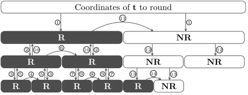
1. Arrows are labeled in their order of execution. Down-ward (↓ ↓) (resp. upDown-ward (↑ ↑)) arrows correspond to computing Vd/d0(tj) (resp. V−1
d/d0(. . .)) at step 9. Transverse (y) arrows correspond to step 8.
2. Cells labeled withR(as in Rounded) correspond to already completed subcalls of Algorithm 4, as opposed to those labeled withNR(as inNotRounded).
Figure 5: High-level execution of the fast Fourier nearest plane algorithm
Unlike the fast Fourier transform, Algorithm 4 is not fully parallelizable, due to step 8 (yarrows in Figure 5). However, its complexity indis Θ(dlogd): informally, this is because each arrow↓,↑ory has a linear complexity in the size of the cells it connects. A more precise statement follows.
Lemma 4. Letd∈Nand1 =d0|d1|. . .|dh=d be be the
tower of proper divisors of d given by the successive gpds, and fori∈J1, hK, letki
∆
=di/di−1. LetB∈ Rn×md andLbe
its LDL?decomposition tree. The complexity of Algorithm 4 is given by:
Θ(ndlogd) + Θ(n2d) + Θ(nd) X
16i6h
k2i.
In particular, if all the ki are bounded by a constant, then
the complexity of Algorithm 4 isΘ(n2d+ndlogd).
The proof of Lemma 4 is deferred to Appendix F.
Acknowledgements
The authors would like to thank the anonymous reviewers of ISSAC and EUROCRYPT for their diligent comments, significantly contributing to improve the presentation of this article.
5.
REFERENCES
[1] Babai, L.On Lov´asz’ lattice reduction and the nearest lattice point problem.Combinatorica 6, 1 (1986), 1–13. Preliminary version in STACS 1985.
[2] Cooley, J. W., and Tukey, J. W.An algorithm for the machine calculation of complex Fourier series.
Mathematics of Computation 19, 90 (1965), 297–301. [3] Durbin, J.The fitting of time-series models.Review of
the International Statistical Institute 28, 3 (1960), pp. 233–244.
[4] Gentleman, W. M., and Sande, G.Fast Fourier transforms: for fun and profit. InProceedings of the November 7-10, 1966, fall joint computer conference
(1966), ACM, pp. 563–578.
[5] Gentry, C., Peikert, C., and Vaikuntanathan, V. Trapdoors for hard lattices and new cryptographic constructions. InSTOC (2008).
[6] Gorbunov, S., Vaikuntanathan, V., and Wee, H.
Attribute-based encryption for circuits. In45th ACM STOC (June 2013), D. Boneh, T. Roughgarden, and J. Feigenbaum, Eds., ACM Press, pp. 545–554. [7] Gragg, W. B.Positive definite toeplitz matrices, the
arnoldi process for isometric operators, and gaussian quadrature on the unit circle.Journal of Computational and Applied Mathematics 46, 1-2 (1993), 183 – 198. [8] Heideman, M. T., Johnson, D. H., and Burrus,
C. S.Gauss and the history of the fast Fourier
transform.ASSP Magazine, IEEE 1, 4 (1984), 14–21. [9] Hoffstein, J., Howgrave-Graham, N., Pipher, J.,
Silverman, J. H., and Whyte, W.NTRUSIGN: Digital signatures using the NTRU lattice. InCT-RSA (2003).
[10] Hoffstein, J., Pipher, J., and Silverman, J. H. NTRU: A ring-based public key cryptosystem. In
ANTS (1998), pp. 267–288.
[11] Klein, P. N.Finding the closest lattice vector when it’s unusually close. InSODA(2000), pp. 937–941. [12] Lang, S.Algebraic number theory, 3 ed. 1995.
[13] Lenstra, A. K., Lenstra, Jr., H. W., and Lov´asz, L.Factoring polynomials with rational coefficients.
Mathematische Annalen 261, 4 (December 1982), 515–534.
[14] Levinson, N.The Wiener RMS (root mean square) error criterion in filter design and prediction.J. Math. Phys. Mass. Inst. Tech. 25 (1947), 261–278.
[15] Lyubashevsky, V., Micciancio, D., Peikert, C., and Rosen, A.SWIFFT: A modest proposal for FFT
hashing. InFSE (2008).
[16] Lyubashevsky, V., Peikert, C., and Regev, O.On ideal lattices and learning with errors over rings. In
EUROCRYPT (2010), pp. 1–23.
[17] Lyubashevsky, V., and Prest, T.Quadratic time, linear space algorithms for Gram-Schmidt
orthogonalization and Gaussian sampling in structured lattices. InEUROCRYPT 2015.
[18] Micciancio, D., and Peikert, C.Trapdoors for lattices: Simpler, tighter, faster, smaller. In
EUROCRYPT (2012).
[19] Nussbaumer, H. J.Fast Fourier transform and convolution algorithms, vol. 2. Springer Science & Business Media, 2012.
[20] Olshevsky, V.Fast Algorithms for Structured Matrices: Theory and Applications, vol. 323. American Mathematical Soc., 2003.
[21] Olshevsky, V., and Pan, V. Y.A unified superfast algorithm for boundary rational tangential
interpolation problems and for inversion and factorization of dense structured matrices. InFOCS (1998).
[22] Peikert, C.An efficient and parallel Gaussian sampler for lattices. InCRYPTO (2010), pp. 80–97.
[23] Sweet, D. R.Fast toeplitz orthogonalization.
APPENDIX
A.
EXTENDING THE RESULTS TO
CYCLO-TOMIC RINGS
In this section we argue that our results hold in the cy-clotomic case as well. It turns out that all the previous arguments can be made more general. The required ingredi-ents are the following:
1. A tower of unitary rings endowed with inner products ontoR.
2. For any ringsS,T of the tower, injective maps M0 : S → Tk×kandV0:S → Tk, withSof rankdover
R, andT of rankd/k overR.
3. M0 is a ring morphism.
4. V0is a scaled linear isometry.
5. V0(ab) =M0(a)V0(b).
6. ComputingV0,V0−1,M0
andM0−1 takes time Θ(dk).
It remains to prove the existence of such maps for towers of cyclotomic rings. We give explicit constructions in this section, using both our maps from the previous sections and a generic embedding from cyclotomic ringsFdto convolution ringsRd.
A.1
Cyclotomic Rings
We give brief reminders about cyclotomic polynomials and rings. Ford ∈N∗,ζd denotes an arbitrary primitive d-th root of unity inC, for exampleζd=e
2iπ
d . Ωd={ζdk|k∈Z× d} denotes the set of primitived-th roots of unity. Let
φd(x) =
Y
ζ∈Ωd
(x−ζ) = Y
k∈Z× d
(x−ζdk).
This polynomial inZ[x] is called thed-th cyclotomic polyno-mial. In addition, we define the polynomialψdas follows:
ψd(x) =
Y
ζd=1,ζ /∈Ωd
(x−ζ) = Y
k∈Zd\Z× d
(x−ζdk).
It is immediate that for any d, the degree ofφdis ϕ(d), whereϕ(d)=∆|Z×d|is Euler’s totient function. One can also check thatφd(x)·ψd(x) =xd−1. To conclude, letFddenote the cyclotomic ringR[x]/(φd(x)).
For additional documentation about cyclotomic polynomi-als, rings and fields, the readers can refer to e.g. [12], Chapter IV.
A.2
Embedding the Ring
F
din the Ring
R
d We now explicit an embedding ofFdintoRd.Definition 10. Leted be the unique element inRdsuch
that ed = 1 modφd and ed = 0 modψd. We define the
embeddingιdfromFdintoRd as follows:
ιd : Fd → Rd
f 7→ f·ed.
When clear from context, we simply noteι=ιd.
Equivalently,ι(f) is the only element inRdsatisfying:
ι(f)(ζ) =
f(ζ) ifφd(ζ) = 0
0 ifψd(ζ) = 0 (4)
Proposition 5. Let d∈N∗and ι=ιd. The embedding
ι:
1. is an injective ring morphism.
2. is an isometry : for anyf, g∈ Fd,hι(f), ι(g)i=hf, gi.
Proof. Item 1 follows from the fact thatedis idempotent
e2
d=ed. Indeed this implies thated(a+bc) =eda+edbc=
eda+e2dbc=eda+ (edb)(edc). In addition, for any element
g ∈ ι(Fd), gmodφd is the unique antecedent of g with respect toι, soιis bijective andι−1(g) =gmodφ
d, which proves the point 1. Item 2 follows from equation (4).
Lemma 5. Letd>2, d0|d, k=d/d0 anda∈ Rd. Then (a∈ι(Fd))⇔Vd/d0(a)∈ι(Fd0)k
Proof. We prove the lemma ford0= gpd(d), extension
to the general case is straightforward. a can be uniquely written asa=P
06i<kx i
ai(xk) where eachai∈ Rd0. Letζd be an arbitraryd-th primitive root of unity. We recall that Ωd={ζdj|j∈Z×d}and noteUd
∆
={ζ∈C|ζd= 1}={ζdj|j∈ Zd}. One can check that
(ζ∈Ud\Ωd)⇔(ζk∈Ud0\Ωd0), (5)
which is immediate by writingζ=ζdj, withj∈Zd\Z×d. We recall that evaluatinga on each ζdj ∈ Ud yields the linear system
a(ζdj) = X
06i<k
ζdijai(ζdkj) =
X
06i<k
ζdijai(ζdj0). (6)
As a step of the FFT (see Lemma 1), the system 6 is invertible. In addition, one can check in equation 5 that if
ζ ∈ Ud\Ωd, thena(ζ) depends only of theai(ζ0) for ζ0 ∈
Ud0\Ωd0. Similarly, ifζ∈Ωd, thena(ζ) depends only of the
ai(ζ0) forζ0∈Ωd0. So the linear system can be separated in
two independent systems. Notinga(E)=∆{a(e)|e∈E}:
a(Ωd) a(Ud\Ωd)
=
(ai(Ωd0))06i<k (ai(Ud0\Ωd0))06i<k
M1 0
0 M2
.
(7)
Since the whole system is invertible, both matricesM1and
M2 are invertible too. We can conclude thata(Ud0\Ωd0) = 0d−ϕ(d) iff all thea
i(Ud0\Ωd0)’s are zero too. This is equiva-lent to saying thata∈ι(Fd) iff∀i, ai∈ι(Fd0), which proves the lemma.
A.3
Conclusion for Cyclotomic Rings
We now check that the 6 conditions enounced at the be-ginning of Section A are verified. For d0|d, Fd0 and Fd0 are unitary rings endowed with the dot product defined in Definition 2, which gives the condition 1. The embeddings
ιdtrivialize the construction of mapsM0andV0 fromFdto Fd0:
V0=ι−d01◦Vd/d0◦ιd M0=ι−1
d0 ◦Md/d0◦ιd.
This gives the condition 2. Lemma 5 allows to argue that the image ofVd/d0◦ιdis in the definition domain ofι−1
d0 : V 0
properties hold for Md/d0 and Vd/d0. Condition 4 is true becauseιd,Vd/d0 andιd0 are isometries. Finally, condition 6 holds in the FFT representation, from Lemma 1 and from the fact thatιin the Fourier domain simply consist of inserting some zeros at appropriate positions.
B.
IMPLEMENTATION IN PYTHON
In this section, we give the core of the Python imple-mentation of our algorithms whend is a power of 2. The full implementation, including correctness tests, is available online and placed in the public domain:
https://github.com/lducas/ffo.py.
Conventions.
Inpython.numpy, the arithmetic operations+, -, ?and
/applied on arrays denote coefficient-wise operations. The functionsfftand its inverseifftare built in. The symbolj
denotes the imaginary unit. The primitivezeros(d)creates thed-dimensional zero vector.
# Simplified extract of ffo.py
from numpy import *
# Linearize operation V, i/o in fft format
def ffsplit(F): d = len(F)
winv = exp(2j*pi / d)
Winv = array([winv**i for i in range(d/2)]) F1 = .5* (F[:d/2] + F[d/2:])
F2 = .5* (F[:d/2] - F[d/2:]) * Winv return (F1,F2)
# Inverse linearize V^-1, i/o in fft format
def ffmerge(F1,F2): d = 2*len(F1)
F = 0.j*zeros(d) # Force F to complex float
w = exp(-2j*pi / d)
W = array([w**i for i in range(d/2)]) F[:d/2] = F1 + W * F2
F[d/2:] = F1 - W * F2 return F
# ffLDL alg., i/o in fft format # Outputs an L-Tree (sec 3.2)
def ffLDL(G): d = len(G) if d==1:
return (G,[]) (G1,G2) = ffsplit(G) L = G2 / G1
D1 = G1
D2 = G1 - L * G1 * conjugate(L) return (L, [ffLDL(D1),ffLDL(D2)] )
# ffLQ, i/o in fft format # outputs an L-Tree (sec 3.2)
def ffLQ(f): F = fft(f)
G = F*conjugate(F) T = ffLDL(G) return T
# ffNearestPlane, i/o in base B, fft format (sec. 4)
def ffBabai_aux(T,t): if len(t)==1:
return array([round(t.real)]) (t1,t2) = ffsplit(t)
(L,[T1,T2]) = T
z2 = ffBabai_aux(T2,t2)
tb1 = t1 + (t2-z2) * conjugate(L) z1 = ffBabai_aux(T1,tb1)
return ffmerge(z1,z2)
# ffNearestPlane, i/o in canonical base, coef. format
def ffBabai(f,T,c): F = fft(f) t = fft(c) / F z = ffBabai_aux(T,t) return ifft(z * F)
C.
PROOF OF PROPOSITION 1
Proof. For anyx,y∈ Rm
, lethx,yiR=∆x·y?. One can check thath·,·iRis a Hermitian inner product. In particular,
(hx,xiR= 0)⇔(hx,xi= 0)⇔(x=0).
The decompositionB=L·B˜ can be computed using the Gram-Schmidt process (Algorithm 5).
Algorithm 5GramSchmidtR(B) 1: fori= 1, . . . , ndo
2: ˜bi←bi
3: forj= 1, . . . , i−1do 4: Li,j=
hbi,b˜jiR h˜b
j,˜bjiR 5: bi˜ ←bi˜ −Li,jbj˜ 6: end for
7: end for
8: return ( ˜B={b˜1, . . . ,bn˜ },L= (Lij)16i,j6n)
If we replaceRwithRor a number field, it is well-known that Algorithm 5 terminates whenever Bis full-rank, and outputs ( ˜B,L) satisfying equation 1. However, it is less obvious in our case, since R is no longer a field and the division byhbj˜ ,bj˜ iRin step 4 might be problematic.
To show that the output of Algorithm 5 satisfies equation 1 when R = R[x]/(h(x)), it suffices to show that for any
j∈J1, nK,hbj˜ ,bj˜ iRis invertible. Suppose that it is not the case, then there existsj∈J1, nK, anda∈ R\{0}such that ahbj˜ ,bj˜ iR= 0. By linearity,habj˜ , abj˜ iR= 0 and therefore
abj˜ = 0. Since ˜bj = bj−P
i<jLi,jbj˜ , this means that there exists a nonzero linear combinationP
i6jaibiequal to zero. ThereforeBis not full-rank, which contradicts the hypothesis of Proposition 1.
Unicity of the decomposition follows from the unicity of the orthogonal projection of a vector onto aR-module.
Our arguments seamlessly transfer to the termination of Algorithm 1, as the elementsDj in Algorithm 1 are exactly the elementshbj˜ ,bj˜ iRin Algorithm 5.
D.
PROOF OF PROPOSITION 4
1. We first prove this statement ford0 = gpd(d) and for elements a, b ∈ Rd. All the requirements for show-ing thatMis a homomorphism are trivial, except for the fact that it is multiplicative. First, one can check from Definition 8 that M(ab) = M(a) ·M(b). Let A = (aij) ∈ Rn×pd and B = (bij) ∈ Rp×md . Since AB= (∆ P
16k6paikbkj)16i6n,16j6m, we have
M(AB) = M
P
16k6paikbkj
i,j
= P
16k6pM(aik)M(bkj)
i,j = M(A)M(B)
.
Multiplicity then seamlessly transfers to anyd00|d:
Md/d00(A·B) = Md0/d00◦Md/d0(A·B) = Md0/d00(Md/d0(A)·Md/d0(B))
= Md0/d00◦Md/d0(A)·Md0/d00◦Md/d0(B) = Md/d00(A)·Md0/d00(B).
To show injectivity, it suffices to see that ifd0= gpd(d), then (Md/d0(a) = 0)⇔(a = 0). From the definition, this property seamlessly transfers to anyd0|dand any matrixA.
2. This item is immediate from the definition.
3. It suffices to notice that for anya,V(a) is the first line ofM(a). AsMis a multiplicative homomorphism, the result follows.
4. It suffices to prove it for elementsa, b∈ Rd (instead of vectors) and ford0 = gpd(d), the generalization to vectors and to arbitrary values ofd0 is then immediate. Leta=P
ix ia
i(xgpd(d)), b=Pix ib
i(xgpd(d)), where ∀i, ai = Pj∈Zgpd(d)ai,jxj and bi = Pj∈Zgpd(d)bi,jxj. Then
ha, bi2∆=X i,j
hai,j, bi,ji2=
X
i
hai, bii2
∆
=hV(a),V(b)i2.
5. We have:
Bfull-rank⇔ ∀a,aB= 0 iffa= 0 ⇔ ∀a,V(aB) = 0 iffV(a) = 0
⇔ ∀a0,V(a0)M(B) = 0 iffV(a0) = 0
⇔ ∀a0,a0M(B) = 0 iffa0= 0 ⇔M(B) full-rank
The first and last equivalences are simply the definition, the second and fourth uses the fact thatVis a vector space isomorphism and the third one uses Proposition 4, item 3.
E.
PROOF OF LEMMA 2
Proof. Let C(k, d) denote the complexity of Algorithm 3
over a matrixG∈ Rk×k
d . We have the following recursion formula:
C(n, d) = Θ(n2dlogd) + Θ(n3d) + Θ(dk2h) +nC(kh, dh−1),
(8) where the first term corresponds to computing the FFT of then2coefficients of G, and the second term to performing
(L,D)←LDLt
Rd(G) in FFT form. For eachi∈J1, nK, we
know from Lemma 1 thatMd/gpd(d)(Dii) can be computed
in time Θ(dk2
h), hence the third term. The last one is for the
nrecursive calls to itself. We then have
C(kh, dh−1) = P 16i6h
d
diΘ(di−1k
3
i) +dd1C(k1, d0)
= Θ(d) P
16i6h
ki2,
(9)
where the first equality is shown by induction using equa-tion 8,except the first term Θ(n2dlogd) which is no longer
relevant since we are already in the Fourier domain. Com-bining equations 8 and 9, we conclude that the complexity of the whole algorithm is
C(n, d) = Θ(n2dlogd) + Θ(n3d) +nC(kh, dh−1)
= Θ(n2dlogd) + Θ(n3d) + Θ(nd) P
16i6h
k2i.
F.
PROOF OF LEMMA 4
Proof. Let C(k, d) denote the complexity of Algorithm 4
over inputt∈ Rk
d. We have this recursion formula:
C(n, d) = Θ(ndlogd) + Θ(n2d) + Θ(ndkh2) +nC(kh, dh−1),
where the first term corresponds to computing the FFT of the
ncoefficients oft, the second term to performing computing thetj’s (step 8) in FFT form, the third one to thencalls toV−1
d/gpd(d),Md/gpd(d) (see Lemma 1) and the fourth one to
thenrecursive calls to itself. We have
C(kh, dh−1) = P 16i6h
d
diΘ(di−1k
3
i) +dd1C(k1, d0)
= Θ(d) P
16i6h
k2
i,
(10)
where the equalities are obtained using the same reasoning as in the proof of Lemma 2. Similarly, we can then conclude that:
C(n, d) = Θ(ndlogd) + Θ(n2d) + Θ(nd) P
16i6h