Hyperfine structure of muonic mesomolecules
td
µ
,
tp
µ
,
dp
µ
in variational method
A.V.Eskin1,∗,V.I.Korobov1,2,∗∗,A.P.Martynenko1,∗∗∗, andV.V.Sorokin1,∗∗∗∗
1Samara National Research University, 34, Moskovskoye shosse, Samara, 443086, Russia 2BLTP JINR, 141980 Dubna, Moscow region, Russia
Abstract.The hyperfine structure of energy levels of muonic molecules tdµ, tpµand dpµis calculated on the basis of stochastic variational method. The basis wave functions are taken in the Gaussian form. The matrix elements of the Hamiltonian are calculated analytically. Vacuum polarization, relativistic and nuclear structure corrections are taken into account to increase the accuracy. For numerical calculation, a computer code is written in the MATLAB system. Numerical values of energy levels of hyperfine structure in muonic molecules tdµ, tpµand dpµare obtained.
1 Introduction
The interest in hydrogen mesomolecular ions is primarily connected with muonic catalysis of nuclear fusion reactions [1]. Precise calculation of fine and hyperfine structure of muonic molecular ions with the inclusion of higher order QED corrections allows us to predict the rates of reactions of their formation and other parameters of theµCF cycle.
We use stochastic variational method [2–4] to calculate energy spectra of hydrogen me-somoleclular ions numerically. Variational method allows us to determine energies of three-body systems with very high accuracy. Random generation of variational parameters prevents possible convergence of the method to a local minimum and gives a much higher flexibility when applied to different three-body systems. In case of hydrogen mesomolecular ions the
choice of variational method is also motivated by comparable masses of all three particles, which does not allow us to use adiabatic approximation effectively.
In this work not only do we calculate ground state energies and hyperfine structure of tdµ, tpµand dpµmesomolecular ions but also include important QED corrections to increase the accuracy. We calculate relativistic, vacuum polarization and nuclear structure corrections to the ground state energy as well as vacuum polarization and Zemach corrections to the hyperfine splitting. Inclusion of these corrections is crucial in achieving precise results. In all formulas throughout the paper we use muon-atomic units (e=mµ==1).
∗e-mail: [email protected] ∗∗e-mail: [email protected] ∗∗∗e-mail: [email protected] ∗∗∗∗e-mail: [email protected]
2 General formalism
To calculate ground state energy and hyperfine structure in muonic molecules tdµ, tpµand dpµwe use stochastic variational method [4]. The trial wave function of muonic molecule
in this approach has Gaussian form. The Gaussian-type basis function with non-zero angular momentum for nonidentical particles is the following:
φL(x,A)=e−12xAxθL(x),
θL(x)=[[[Yl1(x1)Yl2(x2)]L12Yl3(x3)]L123...]LM,
(1)
wherex=(x1, ...,xN−1) are the Jacobi coordinates,Ais a (N−1)×(N−1) positive-defined matrix of variational parameters,Ylm(x)=rlYlm(x). In the case of three nonidentical particles inS-state (L =0, whereLis total angular momentum of particles) basis functions take the
form:
φ0(ρ,λ,A)=e− 1
2[A11ρ2+A22λ2+2A12(ρλ)], (2) whereρ andλ denote two Jacobi coordinates. Knowing the basis functions we can now perform analytical calculation of matrix elements of the Hamiltonian, which is an advantage of the Gaussian basis. The overlap matrix element has the form:
< φ0|φ0>= 8π 3
(detB)3/2. (3)
where elements of matrix B are expressed in terms of matrix A asBi j=Ai j+Ai j. For the
cal-culation of matrix elements of the Hamiltonian we use explicit expressions for potential and kinetic energy operators. In nonrelativistic approximation the Hamiltonian of the molecule without the account of hyperfine structure has the following form in Jacobi coordinates:
ˆ H=−
2
2µ1∆ρ−
2
2µ2∆λ+ e1e2
|ρ| + e1e3
|λ+ m2
m12ρ|
+ e2e3 |λ− m1
m12ρ|
, (4)
whereµ1 = mm11+mm22, µ2 =
(m1+m2)m3
m1+m2+m3,r12 = r1−r2 =ρ,r13 = r1−r3 = λ+
m2
m12ρ, r23 = r2−r3 =λ− m1
m12ρ,e1,e2,e3are charges of the particles. Matrix elements of kinetic energy have the following analytical form:
< φ0|Tˆ|φ0>=− 24π 3 (detB)5/2
2 2µ1Iρ+
2
2µ2Iλ
, (5)
Iρ=A212B11−2A11A12B12+A11(B212+(A11−B11)B22), (6) Iλ=A212B22−2A22A12B12+A22(B212+(A22−B22)B11). (7) For potential energy matrix elements we present the following analytical expressions:
< φ0|Vˆ|φ0>=e1e2I12+e1e3I13+e2e3I23. (8)
I12= 8
√
2π5/2
√
B22detB, I13,23=
8√2π5/2
F13,23
1 (B22F113,23−(F213,23)2)
, (9)
F13,23
1 =B11+B22 (m13,23
2,1 )2 m2
12
∓2B12m
13,23 2,1 m12 , F
13,23
2 =B12∓B22 m13,23
2,1
m12 , (10)
2 General formalism
To calculate ground state energy and hyperfine structure in muonic molecules tdµ, tpµand dpµwe use stochastic variational method [4]. The trial wave function of muonic molecule
in this approach has Gaussian form. The Gaussian-type basis function with non-zero angular momentum for nonidentical particles is the following:
φL(x,A)=e−12xAxθL(x),
θL(x)=[[[Yl1(x1)Yl2(x2)]L12Yl3(x3)]L123...]LM,
(1)
wherex=(x1, ...,xN−1) are the Jacobi coordinates,Ais a (N−1)×(N−1) positive-defined matrix of variational parameters,Ylm(x)=rlYlm(x). In the case of three nonidentical particles inS-state (L =0, whereLis total angular momentum of particles) basis functions take the
form:
φ0(ρ,λ,A)=e− 1
2[A11ρ2+A22λ2+2A12(ρλ)], (2) whereρ andλ denote two Jacobi coordinates. Knowing the basis functions we can now perform analytical calculation of matrix elements of the Hamiltonian, which is an advantage of the Gaussian basis. The overlap matrix element has the form:
< φ0|φ0>= 8π 3
(detB)3/2. (3)
where elements of matrix B are expressed in terms of matrix A asBi j=Ai j+Ai j. For the
cal-culation of matrix elements of the Hamiltonian we use explicit expressions for potential and kinetic energy operators. In nonrelativistic approximation the Hamiltonian of the molecule without the account of hyperfine structure has the following form in Jacobi coordinates:
ˆ H=−
2
2µ1∆ρ−
2
2µ2∆λ+ e1e2
|ρ| + e1e3
|λ+ m2
m12ρ|
+ e2e3 |λ− m1
m12ρ|
, (4)
whereµ1 = mm11+mm22, µ2 =
(m1+m2)m3
m1+m2+m3, r12 = r1−r2 = ρ,r13 = r1−r3 =λ+
m2
m12ρ,r23 = r2−r3 =λ− m1
m12ρ,e1,e2,e3are charges of the particles. Matrix elements of kinetic energy have the following analytical form:
< φ0|Tˆ|φ0>=− 24π 3 (detB)5/2
2 2µ1Iρ+
2
2µ2Iλ
, (5)
Iρ=A212B11−2A11A12B12+A11(B212+(A11−B11)B22), (6) Iλ=A212B22−2A22A12B12+A22(B212+(A22−B22)B11). (7) For potential energy matrix elements we present the following analytical expressions:
< φ0|Vˆ|φ0 >=e1e2I12+e1e3I13+e2e3I23. (8)
I12= 8
√
2π5/2
√
B22detB, I13,23=
8√2π5/2
F13,23
1 (B22F131 ,23−(F213,23)2)
, (9)
F13,23
1 =B11+B22 (m13,23
2,1 )2 m2
12
∓2B12m
13,23 2,1 m12 , F
13,23
2 =B12∓B22 m13,23
2,1
m12 , (10)
where to get the expressions forF13
1 andF132 one should choosem2and the first sign in (10) and to obtainF23
1 andF223m1and the second sign in (10) must be chosen.
To further increase the accuracy of our calculation we take into account various QED corrections. Let us start with relativistic corrections. The explicit expression for relativistic corrections can be obtained from the Breit Hamiltonian for two interacting particles. In case of hydrogen mesomolecular ions Breit corrections have the form [5, 6]:
VB=−α 2 8 3 i=1 p4 i m3 i
−πα22
3
i,j=1;ij
eiej
1 m2 i + 1 m2 j
δ(ri j)−α
2 2
3
i,j=1;ij
eiej
pipj+
ri j(ri j·pi)pj
r2 i j
mimjri j ,
(11) wherepiare momentums of the particles,ri j =ri−rjare interparticle coordinates. Averaging over basis functions gives the following analytical expressions for matrix elements:
< φi|p41|φj>= 15(2π)
3
(detB)7/2
A11j +2 m1 m1+m2A
j
12+
m1
m1+m2 2
A22j ×
×det(Ai)+Ai
11+2m1m1+m2Ai12+
m1
m1+m2 2
Ai
22
det(Aj)2, (12)
< φi|p42|φj>= 15(2π)
3
(detB)7/2
A11j −2 m2 m1+m2A
j
12+
m2
m1+m2 2
A22j ×
×det(Ai)+Ai
11−2 m2 m1+m2A
i
12+
m2
m1+m2 2
Ai
22
det(Aj)2, (13)
< φi|p43|φj>= 15(2π)
3
(detB)7/2[A
j
22detAi+Ai22detAj]2, (14)
< φi|r1
12
p1p2+r12(r12r2·p1)p2 12
|φj>= 8(2π)
5/2
[√B22(detB)2]
Ai
11+
m1−m2 m1+m2A
i
12− (15)
−(mm1m2
1+m2)2A
i
22
det(Aj)+Aj
11+
m1−m2 m1+m2A
j
12−
m1m2 (m1+m2)2A
j
22
det(Ai),
< φi| 1
r13
p1p3+ r13(r13r2·p1)p3 13
|φj>= 8(2π)
5/2
(detB)2
B11−2 m2
m1+m2B12+
m2
m1+m2 2
B22
× (16)
×m m1
1+m2A
i
22+Ai12
det(Aj)+ m1
m1+m2A
j
22+A12j
det(Ai),
< φi| 1
r23
p2p3+ r23(r23r2·p2)p3 23
|φj>= 8(2π)
5/2
(detB)2
B11+2 m1
m1+m2B12+
m1
m1+m2 2
B22
× (17)
×m1m+2m2Ai22−Ai12det(Aj)+ m2
m1+m2A
j
22−A
j
12
det(Ai).
Now let us consider another important QED correction - one-loop vacuum polarization correction. The potential in this case takes the form:
VVP= α
3π
3
i,j=1;ij
eiej
ri j
∞
1 dξρ(ξ)e
−2γξri j, (18)
whereγ= me
mµα,ρ(ξ)=
ξ2−1(2ξ2+1)/ξ4. Analytical expression for matrix elements is the
following:
< φi| 1
r12 ∞
1 dξ
ξ2−1(2ξ2+1)
ξ4 e
−2me
mµ αξr12|φj>=
√
2π7/2 4M5/2B3/2
22
×
×8πM3/2G2,1 3,4
γ2
M| 0,12,32
0,0,12,12
+ √π(4√πM3/2G2,1 3,4
γ2
M| 0,12,52
0,1,12,12
+8γ3+12γM),
(19)
< φi| 1
r13,23 ∞
1 dξ
ξ2−1(2ξ2+1)
ξ4 e
−2me
mµ αξr13,23|φj>=
=
√
2π7/2 4(L13,23)5/2(F13,23
1 )3/2
×8π(L13,23)3/2G23,,14
γ2
L13,23| 0,12,32
0,0,12,12
+
+√π(4√π(L13,23)3/2G2,1 3,4
γ2
L13,23| 0,12,52
0,1,12,12
+8γ3+12γL13,23),
(20)
L= B22F 13,23
1 −(F213,23) 2F13,23
1
, M=detB
2B22, (21)
whereGis the Meijer G-function.
It is important to also include nuclear structure correction, which in case of mesomolec-ular ions has the form:
Vstr=−2
3π(e1e3)r21eδ3(r13)−32π(e2e3)r22eδ3(r23), (22) where indices 1, 2 denote nuclei of hydrogen isotopes,r1e, r2eare charge radii of the
cor-responding nuclei of hydrogen isotopes, index 3 denotes the muon. This correction can be obtained using the following expansion of electric form-factor:
GE(k2)|k2→0=GE(0)+dGE(k 2) dk2 k2=0k
2+...=1−1
6rE2k2+... (23)
The calculation of the matrix elements ofδ3(ri j) will be presented explicitly in the next
sec-tion. To calculate QED corrections numerically we use first order perturbation theory. Gen-eral expression for an arbitrary potential:
<V >=
K
i,j=1cicj< φi|V|φj>
K
i,j=1cicj[(Ai 8π3
11+A11j)(Ai22+A22j)−(Ai12+A12j)2]3/2
, (24)
whereVis an arbitrary potential,ci,cjare linear variational parameters,Kis the number of
basis functions. All numerical results for ground state energy and corrections after variational calculation are presented in Table 1 in lines 1 through 4. Results from paper [3] are presented in Table 1 in parentheses for comparison.
3 Hyperfine structure
Now let us calculate matrix elements of the hyperfine part of the Hamiltonian. The potential of hyperfine structure ofL=0 state, which is a part of the Breit Hamiltonian, can be written
in the following simple form for three interacting particles with spinsS1,S2,S3respectively [7–9]:
∆Vh f s=a(S1S2)+b(S1S3)+c(S2S3), (25)
whereγ= me
mµα,ρ(ξ)=
ξ2−1(2ξ2+1)/ξ4. Analytical expression for matrix elements is the
following:
< φi| 1
r12 ∞
1 dξ
ξ2−1(2ξ2+1)
ξ4 e
−2me
mµ αξr12|φj>=
√
2π7/2 4M5/2B3/2
22
×
×8πM3/2G2,1 3,4
γ2
M| 0,12,32
0,0,12,12
+ √π(4√πM3/2G2,1 3,4
γ2
M| 0,12,52
0,1,12,12
+8γ3+12γM),
(19)
< φi| 1
r13,23 ∞
1 dξ
ξ2−1(2ξ2+1)
ξ4 e
−2me
mµ αξr13,23|φj>=
=
√
2π7/2 4(L13,23)5/2(F13,23
1 )3/2
×8π(L13,23)3/2G23,,14
γ2
L13,23| 0,12,32
0,0,12,12
+
+√π(4√π(L13,23)3/2G2,1 3,4
γ2
L13,23| 0,12,52
0,1,12,12
+8γ3+12γL13,23),
(20)
L= B22F 13,23
1 −(F213,23) 2F13,23
1
, M=detB
2B22, (21)
whereGis the Meijer G-function.
It is important to also include nuclear structure correction, which in case of mesomolec-ular ions has the form:
Vstr=−2
3π(e1e3)r12eδ3(r13)−32π(e2e3)r22eδ3(r23), (22) where indices 1, 2 denote nuclei of hydrogen isotopes,r1e, r2e are charge radii of the
cor-responding nuclei of hydrogen isotopes, index 3 denotes the muon. This correction can be obtained using the following expansion of electric form-factor:
GE(k2)|k2→0=GE(0)+dGE(k 2) dk2 k2=0k
2+...=1−1
6r2Ek2+... (23)
The calculation of the matrix elements ofδ3(ri j) will be presented explicitly in the next
sec-tion. To calculate QED corrections numerically we use first order perturbation theory. Gen-eral expression for an arbitrary potential:
<V>=
K
i,j=1cicj< φi|V|φj>
K
i,j=1cicj[(Ai 8π3
11+A11j )(Ai22+A22j)−(Ai12+A12j)2]3/2
, (24)
whereVis an arbitrary potential,ci,cjare linear variational parameters,Kis the number of
basis functions. All numerical results for ground state energy and corrections after variational calculation are presented in Table 1 in lines 1 through 4. Results from paper [3] are presented in Table 1 in parentheses for comparison.
3 Hyperfine structure
Now let us calculate matrix elements of the hyperfine part of the Hamiltonian. The potential of hyperfine structure ofL=0 state, which is a part of the Breit Hamiltonian, can be written
in the following simple form for three interacting particles with spinsS1,S2,S3respectively [7–9]:
∆Vh f s=a(S1S2)+b(S1S3)+c(S2S3), (25)
a=−2πα 2g
1g2 3m2
p
δ3(r12), b= 2πα 2g
1g3 3mp δ
3(r
13), c=2πα
2g 2g3 3mp δ
3(r
23),
whereg1,g2,g3 are gyromagnetic factors, indices 1,2 denote nuclei of hydrogen isotopes, index 3 denotes muon. Averaging procedure for such potential involves both averaging over radial and spin basis functions. Analytical integration of radial matrix elements ofδ(ri j) can be performed as follows:
< δ3(r12)>=< δ(ρ)>= dρdλδ(ρ)e−12[B11ρ2+B22λ2+2B12(ρλ)]=
=4π
λ2dλδ(ρ)e−21B22λ2= (2π) 3/2
(B22)3/2. (26)
< δ3(r13)>= (2π) 3/2 (B11−2B12mm122+B22(
m2
m12)
2)3/2, (27)
< δ3(r23)>= (2π) 3/2
(B11+2B12mm112+B22(
m1
m12)
2)3/2. (28)
To perform averaging over spin functions Wigner - Eckart theorem [10] can be used with success. General formulas for spin averaging for anyS1,S2andS3take the form:
<S12,S|(S1S2)|S12,S >=(S1S2)S12δS12S12, (29)
<S12,S|(S1S3)|S12,S >=
(2S
12+1)(2S12+1)(2S1+1)(S1+1)S1
(2S3+1)×
×(S3+1)S3(−1)Smax12 +Smin12+S+S1+S2+S3+1 S12 S3 S S3 S12 1
S
1 S12 S2 S12 S1; 1
, (30)
<S12,S|(S2S3)|S12,S >=
(2S
12+1)(2S12+1)(2S2+1)(S2+1)S2
(2S3+1)×
×(S3+1)S3(−1)2S max
12 +S+S1+S2+S3+1 S12 S3 S S3 S12 1
S
2 S12 S1 S12 S2 1
. (31)
In the case ofS1=S2=S3=1/2 the energy matrix has the form:
14a+14b+14c 0 0
0 1
4a−12b−12c
√
3 4 b−
√
3 4 c
0 √3
4 b−
√
3
4 c −34a
. (32)
After the matrix diagonalization we obtain the following eigenvalues:
λ1,2 =−14(a+b+c)±12√a2+b2+c2−ab−bc−ac, λ3=14(a+b+c). (33)
These eigenvalues are energies of hyperfine structure levels with respect to the total energy of ground state. In case ofS1 = S2 = S3 = 1/2, as it was already mentioned, we have 3 hyperfine levels. In the case ofS1=1, S2=S3=1/2 the energy matrix is the following:
1
2a+12b+14c 0 0 0
0 1
2a−56b−125c
√
2 3 b−
√
2
3 c 0
0 √2
3 b−
√
2
3 c −a+13b−121c 0
0 0 0 −a−b+14c
. (34)
After the matrix diagonalization the following eigenvalues are obtained:
λ1= 14(−4a−4b+c), λ2= 14(2a+2b+c), (35)
λ3,4=14(∓
9a2−14ab−4ac+9b2−4bc+4c2−a−b−c). (36)
ForS1 = 1, S2 = S3 = 1/2 spin configuration we get 4 hyperfine levels. To calculate hyperfine structure of muonic molecular ions tdµ, tpµ, dpµwe use first order perturbation theory with a variational wave function obtained in variational calculation. For instance, to calculate< δ(r12) >matrix element in first order perturbation theory one has to use the following expression:
< δ(r12)>=
K
i,j=1cicj (2π)
3/2 (Ai
22+A22j)3/2 K
i,j=1cicj[(Ai 8π3
11+A11j )(Ai22+A22j)−(Ai12+A12j)2]3/2
. (37)
Other matrix elements are evaluated in a similar way. Thus we obtain numerical values ofa, bandccoefficients and energies of hyperfine structure levels of tdµ, tpµ, dpµmesomolecular
ions.
To obtain a more precise result we include vacuum polarization and nuclear structure corrections to hyperfine structure. The potential of one loop vacuum polarization correction to the hyperfine structure has the form:
∆VVPh f s=aVP(S1S2)+bVP(S1S3)+cVP(S2S3), (38)
aVP=−2α
2g 1g2 3m2
p
α
3π
∞
1 ρ(ξ)dξ
πδ(r12)−γr122ξ2e−2γξr12,
bVP= 2α
2g 1g3 3mpm3
α
3π
∞
1 ρ(ξ)dξ
πδ(r13)−γ
2ξ2
r13 e−2
γξr13
,
cVP=2α
2g2g3 3mpm3
α
3π
∞
1 ρ(ξ)dξ
πδ(r23)−γ
2ξ2 r23 e
−2γξr23
.
Integration over the Jacobi coordinates can be performed analytically. Thus we obtain the following integral expressions for vacuum polarization correction to the hyperfine structure:
I12
VP,h f s=
∞
1 ρ(ξ)dξ
2√2π5/2 B3/2
22
−
−
8π2γ2ξ2
√2π
B11−B212
B22 −2πγξe
2B22γ2ξ2
B11B22−B212erfc√2γξ B22
B11B22−B212
B11B22−B2 12
3/2
,
(39)
I13,23
VP,h f s=
∞
1 ρ(ξ)dξ
2√2π5/2 (F13,23
1 )3/2
− 8π2γ2ξ2
F13,23
1 B22−(F213,23)2 3/2
√ 2π
B22− (F13,23
2 )2 F13,23
1
−
−2πγξe 2F13,23
1 γ2ξ2
F131,23B22−(F132,23)2erfc(√2γξ
F13,23 1 F13,23
1 B22−(F213,23)2 ),
(40)
After the matrix diagonalization the following eigenvalues are obtained:
λ1=14(−4a−4b+c), λ2= 14(2a+2b+c), (35)
λ3,4=14(∓
9a2−14ab−4ac+9b2−4bc+4c2−a−b−c). (36)
ForS1 = 1, S2 = S3 = 1/2 spin configuration we get 4 hyperfine levels. To calculate hyperfine structure of muonic molecular ions tdµ, tpµ, dpµwe use first order perturbation theory with a variational wave function obtained in variational calculation. For instance, to calculate< δ(r12) >matrix element in first order perturbation theory one has to use the following expression:
< δ(r12)>=
K
i,j=1cicj (2π)
3/2 (Ai
22+A22j)3/2 K
i,j=1cicj[(Ai 8π3
11+A11j)(Ai22+A22j)−(Ai12+A12j)2]3/2
. (37)
Other matrix elements are evaluated in a similar way. Thus we obtain numerical values ofa, bandccoefficients and energies of hyperfine structure levels of tdµ, tpµ, dpµmesomolecular
ions.
To obtain a more precise result we include vacuum polarization and nuclear structure corrections to hyperfine structure. The potential of one loop vacuum polarization correction to the hyperfine structure has the form:
∆VVPh f s=aVP(S1S2)+bVP(S1S3)+cVP(S2S3), (38)
aVP=−2α
2g 1g2 3m2
p
α
3π
∞
1 ρ(ξ)dξ
πδ(r12)−γr122ξ2e−2γξr12,
bVP= 2α
2g 1g3 3mpm3
α
3π
∞
1 ρ(ξ)dξ
πδ(r13)−γ
2ξ2
r13 e−2
γξr13
,
cVP=2α
2g2g3 3mpm3
α
3π
∞
1 ρ(ξ)dξ
πδ(r23)−γ
2ξ2 r23 e
−2γξr23
.
Integration over the Jacobi coordinates can be performed analytically. Thus we obtain the following integral expressions for vacuum polarization correction to the hyperfine structure:
I12
VP,h f s=
∞
1 ρ(ξ)dξ
2√2π5/2 B3/2
22
−
−
8π2γ2ξ2
√2π
B11−B212
B22 −2πγξe
2B22γ2ξ2
B11B22−B212erfc√2γξ B22
B11B22−B212
B11B22−B2 12
3/2
,
(39)
I13,23
VP,h f s=
∞
1 ρ(ξ)dξ
2√2π5/2 (F13,23
1 )3/2
− 8π2γ2ξ2
F13,23
1 B22−(F213,23)2 3/2
√ 2π
B22− (F13,23
2 )2 F13,23
1
−
−2πγξe 2F13,23
1 γ2ξ2
F131,23B22−(F132,23)2erfc(√2γξ
F13,23 1 F13,23
1 B22−(F213,23)2 ),
(40)
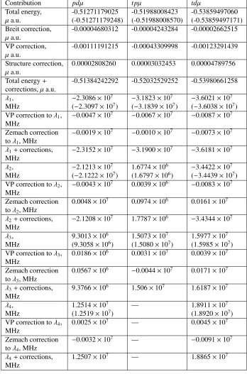
Table 1.Numerical results for hydrogen mesomolecular ions. Numerical values for ground state and hyperfine structure as well as QED corrections are presented. In parenthesis numerical results from [3]
are presented
Contribution pdµ tpµ tdµ
Total energy, -0.51271179025 -0.51988008423 -0.53859497060
µa.u. (-0.51271179248) (-0.51988008570) (-0.53859497171)
Breit correction, -0.00004680312 -0.00004243284 -0.00002662515
µa.u.
VP correction, -0.00111191215 -0.00043309998 -0.00123291439
µa.u.
Structure correction, 0.00002808260 0.00003032453 0.00004789756
µa.u.
Total energy+ -0.51384242292 -0.52032529252 -0.53980661258
corrections,µa.u.
λ1, −2.3086×10⁷ −3.1823×10⁷ −3.6021×10⁷ MHz (−2.3097×10⁷) (−3.1839×10⁷) (−3.6038×10⁷) VP correction toλ1, −0.0047×10⁷ −0.0067×10⁷ −0.0087×10⁷ MHz
Zemach correction −0.0019×10⁷ −0.0010×10⁷ −0.0073×10⁷ toλ1, MHz
λ1+corrections, −2.3152×10⁷ −3.1900×10⁷ −3.6181×10⁷ MHz
λ2, −2.1213×10⁷ 1.6774×10⁶ −3.4422×10⁷ MHz (−2.1222×10⁷) (1.6797×10⁶) (−3.4439×10⁷) VP correction toλ2, −0.0043×10⁷ 0.0039×10⁶ −0.0083×10⁷ MHz
Zemach correction 0.0048×10⁷ 0.0974×10⁶ 0.0161×10⁷ toλ2, MHz
λ2+corrections, −2.1208×10⁷ 1.7787×10⁶ −3.4344×10⁷ MHz
λ3, 9.3013×10⁶ 1.5073×10⁷ 1.5977×10⁷ MHz (9.3058×10⁶) (1.5080×10⁷) (1.5985×10⁷) VP correction toλ3, 0.0186×10⁶ 0.0031×10⁷ 0.0039×10⁷ MHz
Zemach correction 0.0567×10⁶ −0.0044×10⁷ 0.0171×10⁷ toλ3, MHz
λ3+corrections, 9.3766×10⁶ 1.506×10⁷ 1.6187×10⁷ MHz
λ4, 1.2514×10⁷ — 1.8911×10⁷ MHz (1.2519×10⁷) (1.8920×10⁷) VP correction toλ4, 0.0025×10⁷ — 0.0045×10⁷ MHz
Zemach correction −0.0032×10⁷ — −0.0091×10⁷ toλ4, MHz
λ4+corrections, 1.2507×10⁷ — 1.8865×10⁷ MHz
where erfc(z) is the complementary error function. Another important correction to the hy-perfine structure of the same order is the well-known Zemach correction. For mesomolecular ions we obtain the following formula for this correction:
∆Vstrh f s,2γ =bstr(S1S3)+cstr(S2S3), (41)
bstr =2α
2g 1g3 3mp δ(r13)
8αm3
π
∞
0 dk k2
G1
E(k2)G1M(k2)
G1
M(0)
−1, (42)
cstr= 2α
2g 2g3 3mp δ(r23)
8αm3
π
∞
0 dk k2
G2
E(k2)G2M(k2)
G2
M(0) −
1. (43)
All numerical values that are calculated in this work are presented in Table 1.
4 Summary and conclusion
For numerical calculation a computer code is written in the MATLAB system to solve the three-body Coulomb problem based on the Schrödinger equation. The Varga-Suzuki program [4] written in Fortran is taken as the basis. Overlap matrix elements, matrix elements of kinetic and potential energies are inserted into the program. The random number generation algorithm has been changed. For variational parameters the stochastic optimization procedure is being used. As a result, the numerical values of the ground state energy as well as energy levels of hyperfine structure of tdµ, tpµ, dpµare obtained. In first order perturbation theory relativistic, vacuum polarization and nuclear structure corrections to the ground state energy are calculated for tdµ, tpµand dpµhydrogen mesomolecular ions. Vacuum polarization and Zemach corrections are taken into account in the hyperfine structure of mesomolecular ions. All energies are in agreement with [3, 11, 12]. The values of ground state energies coincide with the results from paper [3] in 8 digits. In our method we can obtain up to 10 precise digits in ground state energy value which gives us 3 precise digits in hyperfine structure values. The difference in precision with [3] is connected with smaller basis size in our work and lower
convergence rate of the Gaussian basis compared with exponential basis that is used in [3]. It is also worth mentioning that in our calculations we use double precision while in [3] quadruple precision is being used. This fact also contributes to differences in results.
This work is supported by Russian Science Foundation (Grant 18-12-00128).
References
[1] S.S. Gershtein, Yu.V. Petrov, L.I. Ponomarev, Sov. Phys. Usp.33(8), 3 (1990) [2] A.M. Frolov, D.M. Wardlaw, Eur. Phys. J. D63, 339 (2011)
[3] A.M. Frolov, Eur. Phys. J. D66, 212 (2012)
[4] K. Varga, Y. Suzuki, Comp. Phys. Comm.106, 157 (1997) [5] R.N. Faustov et al., Phys. Rev. A92, 052512 (2015) [6] R.N. Faustov et al.,Phys. Rev. A90, 012520 (2014) [7] V.I. Korobov et al., Phys. Part. Nuclei50, 633 (2019)
[8] A.P. Martynenko et al., Bull. Lebedev Phys. Inst.46, 143 (2019) [9] A.V. Eskin et al., EPJ Web of Conferences204, 05006 (2019)
[10] L.D. Landau, E.M. Lifshitz,Quantum Mechanics: Non-Relativistic Theory(Pergamon Press, 1977)
[11] Chi-Yu Hu, Phys. Rev. A32, 1245 (1985)
[12] K. Szalewicz, H.J. Monkhorst, W. Kolos, A. Scrinzi, Phys. Rev. A36, 5494 (1987)