Article A QUBO model for the Traveling Salesman Problem with Time Windows for execution on the D-Wave

Article

A QUBO model for the Traveling Salesman Problem

with Time Windows for execution on the D-Wave

Christos Papalitsas* , Theodore Andronikos*, Konstantinos Giannakis* , Georgia Theocharopoulou, and Sofia Fanarioti

1

2

3

4

5

6

7

DepartmentofInformatics,IonianUniversity,TsirigotiSquare7,Corfu,49100,Greece; {kgiann,c14papa,zeta.theo,sofiafanar,andronikos}@ionio.gr

* Correspondence:[email protected](Ch.P.);[email protected](Th.A.);[email protected](K.G.); ‡ Theseauthorscontributedequallytothiswork.

Abstract: ThisworkfocusesonexpressingtheTSPwithTimeWindows(TSPTWfor short)asa quadraticunconstrainedbinaryoptimization(QUBO)problem. Thetimewindowsimposetime constraintsthatafeasiblesolutionmustsatisfy.Thesetaketheformofinequalityconstraints,which areknowntobeparticularlydifficulttoarticulatewithintheQUBOframework.Thisis,webelieve, thefirsttimethismajorobstacleisovercomeandtheTSPTWiscastintheQUBOformulation.We haveeveryreasontoanticipatethatthisdevelopmentwillleadtotheactualexecutionofsmallscale TSPTWinstancesontheD-Waveplatform.

Keywords:TSP;TSPTW;Metaheuristics;QuantumAnnealing;IshingModel;QUBO;D-Wave 8

1. Introduction 9

Quantum computing promotes the exploit of quantum-mechanical principles for computation 10

purposes. Richard Feynman in 1982 suggested that computation could be done more efficiently by 11

taking advantage of the power of quantum “parallelism” [1]. Since then quantum computing has 12

gained a lot of momentum and today appears to be one of the most prominent candidates to partially 13

replace classical, silicon-based systems. There exist a number of quantum algorithms that run more 14

efficiently than the best known classical algorithm; arguably, the most famous ones are Shor’s [2] and 15

Grover’s [3] algorithms. For an in-depth study of quantum computing and quantum information, the 16

reader is referred to [4]. 17

When solving large scale optimization problems, one of the most effective classical strategies is to 18

search among the nearest neighbors and search for paths between the initial and final configurations 19

to improve upon an initial guessyt. This search takes place locally among neighboring configurations 20

similar toyt. By finding the best solution within the local neighborhood ofyt, the next candidate 21

solutionyt+1appears. Then a new local search starts withyt+1as the starting point in the neighborhood. 22

Unfortunately, greedy local improvement, in case of hard problems, may be deceptively leading the 23

solution into a local minima whose energy may be much higher than the globally minimum value. 24

Adiabatic quantum computation was proposed by Farhi et al. [5,6] in the early 2000s [7] and is 25

based on an important theorem of quantum mechanics, the adiabatic theorem [8,9]. This theorem 26

dictates that if a quantum system is driven by a slowly changing (in time) Hamiltonian that evolves 27

fromHinittoHf in, then if the systems starts in the ground state ofHinit, the system will end up in the 28

ground state ofHf in. Farhi et al. also showed that adiabatic quantum computation can be efficiently 29

simulated by a quantum computer based on the gate model, meaning that the two computational 30

models have the same expressive power [5,6]. 31

Quantum annealing is based on the quantum adiabatic computation paradigm. Quantum 32

annealing was initially proposed by Kadowaki and Nishimori [10,11] and has since then been used 33

for tackling combinatorial optimization problems. The way that a quantum annealer tries to solve 34

problems, is very similar to the way optimization problem are solved using (classical) simulated 35

annealing [12]. An energy landscape is constructed, via a multivariate function, such that the ground 36

state’s coordinates (i.e., the lowest value) correspond to the solution of the problem. The quantum 37

annealing process is iterated to the point that an optimal solution, with a sufficient high probability, is 38

found. The “quantum” in “quantum annealer” refers to the use of multi qubit tunneling [10,11]. The 39

high degree of parallelism is the advantage of quantum annealing over classical code execution. A 40

quantum annealer explores all possible inputs in parallel to find the optimal solution to a problem, 41

which might prove crucial when it comes to solving NP-complete problems. We caution the reader 42

however that, at present, these techniques should be considered more as an automatic heuristic-finding 43

program than as a formal solver [13]. 44

The preceding facts explain why optimization problems have been associated with quantum 45

computing principles [14–18]. In this approach, which can be considered as an “analog” method to 46

tackle optimization problems, the ground state of a Hamiltonian represents an optimal solution of the 47

optimization problem at hand. Typically, the quantum annealing process starts with the system being 48

in an equal superposition of all states. Then, an appropriate Hamiltonian is applied and the system 49

evolves in a time-dependent manner according to the Schrödinger equation. The state of the system 50

keeps changing according to strength of the local transverse field, which varies with respect to time. 51

Finally, the transverse field is smoothly turned off and the system finds itself in the ground state of a 52

properly chosen Hamiltonian that encodes an optimal solution of the optimization problem. 53

After the first commercial launch of an actual system whose functionality is based upon quantum 54

annealing, the D-Wave platform, it has been demonstrated that these particular quantum machines 55

are capable of solving certain quadratic unconstrained (mainly binary) optimization problems. The 56

core of D-Wave’s machine that applies the quantum annealing principles for complex combinatorial 57

optimization problems is the quantum processing unit (QPU). In the D-Wave computer the quantum 58

bits (which we shall refer to as qubits from now on) are the lowest energy states of superconducting 59

loops [7,19,20]. In these states there is a circulating current and a corresponding magnetic field. Since a 60

qubit is a quantum object, its state can be a superposition of the 0 state and the 1 state at the same time. 61

However, upon measurement a qubit collapses to the state 0 or 1 and behaves like a classical bit. The 62

quantum annealing process in effect guides the qubits from a superposition of states to their collapse 63

into either the 0 or 1 state. In the end, the net effect is that the system is in a classical state, which must 64

encode an (optimal) solution of the problem. 65

The current generation of D-Wave computers employs the Chimera topology. In the Chimera 66

topology, qubits are sets of connected unit cells, that are connected to four vertical qubits via 67

couplers [20–22]. The unit cells are oriented vertically and horizontally with adjacent qubits connected, 68

creating a network of sparsely connected qubits. A Chimera graph consists of anN×Ngrid of unit 69

cells. The D-Wave 2000Q QPU has up to 2048 qubits which are mapped to a C16 Chimera graph, that is 70

they are logically mapped into a 16×16 matrix of unit cells, each consisting of 8 qubits. In the D-Wave 71

nomenclature the percentage of working qubits and couplers is known as the working graph, which is 72

typically a subgraph of the total number of interconnected qubits, which are physically present in the 73

QPU. 74

A major category of optimization problems, particularly amenable to D-Wave’s quantum 75

annealing, are those that can be expressed as quadratic unconstrained binary optimization (QUBO) 76

problems. QUBO refers to a pattern matching technique, that, among other applications, can be 77

used in machine learning and optimization, and which involves minimizing a quadratic polynomial 78

over binary variables [20,23–29]. We emphasize that QUBO is NP-hard [29]. Some of the most 79

famous combinatorial optimization problems that can be solved as QUBO problems are the Maximum 80

and related results (that are beyond the scope of this paper) can be found in the survey paper of 82

Kochenberger [25]. QUBO is equivalent to the Ising model, a well-known and extensively studied 83

model in physics, that was introduced in the mid 1920s by Ernst Ising and Wilhelm Lenz in the field 84

of ferromagnetism [31,32]. The underlying logical architecture of this model is that variables are 85

represented as qubits and interactions among qubits stand for the costs associated with each pair of 86

qubits. In particular, this architecture can be depicted as an undirected graph with qubits as vertices 87

and couplers as edges among them. The open-source software qbsolv that D-Wave introduced in 88

2017 is aimed at tackling QUBO problems of higher scale than previous attempts, by utilizing a more 89

complex graph structure with higher connectivity among QPUs, by partitioning the input into parts 90

that are then independently solved. This process is repeated using a Tabu-based search until no further 91

improvement is found [19,33]. 92

The literature contains several works that are dedicated to solving the standard TSP or some 93

relative problem in a quantum setting. One of the first, was the work by Marto ˇnák et al. in [34] 94

that introduced a different quantum annealing scheme based on path-integral Monte Carlo processes 95

to address the symmetric version of the Traveling Salesman Problem (sTSP). In [35,36] the D-Wave 96

platform was used as a test bed for evaluating the efficiency of quantum annealing in solving the 97

standard TSP compared to classical methods. In [37,38] the well-known variation of the TSP, the 98

(Capacitated) Vehicle Routing Problem is studied using, again, the D-Wave computer. However, no 99

work is known to us that tackles the TSP with Time Windows within the QUBO framework, using the 100

D-Wave platform, or even quantum annealing in general. 101

Contribution. In this paper we give the first, to the best of our knowledge, QUBO formulation for 102

the TSP with Time Windows (TSPTW). The existence of an Ising or QUBO formulation for a problem 103

is the essential precondition for its solution on the current generation of D-Wave computers. For the 104

vanilla TSP there exists such a formulation, as presented in an elegant and comprehensive manner 105

in [32], which has enabled the actual solution of TSP instances on the D-Wave platform (see [35–37]). 106

In contrast, prior to this work, the TSPTW had not been cast in the QUBO framework. This can be 107

attributed to the extra difficulty of expressing the time window constraints of TSPTW. We hope and 108

expect that the formulation presented here will lead to the experimental execution of small-scale 109

TSPTW instances. 110

This paper is organized as follows. The most relevant to our study work is presented in Section2. 111

Section3is devoted to the standard definitions and notation of the conventional Traveling Salesman 112

Problem with Time Windows. Section4, the most extensive section of this article, contains the main 113

contribution of our paper. It includes an in-depth presentation of all the required rigorous mathematical 114

definitions and the proposed modeling that allows us to map the TSPTW into the QUBO framework. 115

Finally, conclusions and ideas for future work are given in Section5. 116

2. Related work 117

Quantum annealing [5,11] has been shown to provide solutions to a broad range of combinatorial 118

optimization problems, not only in computer science [6,16,26,30,39–41], but also in other fields, such as 119

quantum chemistry [42], protein folding [14], vehicle routing [33,38,43,44], etc. This kind of problems 120

aim at minimizing a cost function, which can be interpreted as finding the ground state of a typical 121

Ising Hamiltonian [32]. Nevertheless, it is a laborious task to compute a global minimum in problems 122

where multiple local minima exist [45–47], a fact that shares a lot of similarities to classical spin glasses 123

[45,46]. 124

The possible superiority of quantum computation could be translated into either providing a 125

better solution (i.e., closest to the optimal one) or arriving at a solution faster or producing a diverse 126

set of solutions (for the multiobjective case). Some known cases where such methods work well 127

are spin glasses [48], graph coloring [49], job-shop scheduling [50], machine learning [16,51], graph 128

partitioning [30], 3-SAT [52], vehicle routing and scheduling [33,38,43,44], neural networks [53], image 129

Battaglia et al. showed that quantum annealing techniques could outperform their classical 131

counterparts on a known NP-complete problem, the 3-SAT, under special circumstances, whereas 132

in the general case, the quantum versions did not offer any actual advantage [52]. In a recent work, 133

Pagano et al. built a mechanism that implements a shallow-depth quantum approximate optimization 134

algorithm (QAOA) by estimating the ground state energy of the Ising model using an analogue 135

quantum simulator [54]. Farhi and Harrow tried to show the advantages of quantum approximate 136

optimization algorithms compared to classical approaches, providing useful theoretical results and 137

bounds, with the emphasis on the idea of “quantum supremacy” than can be established through such 138

solutions [55]. Constrained polynomial optimization problems using adiabatic quantum computation 139

methods were recently discussed by Rebentrost in [18]. In [56], Venegas-Andraca et al. introduced 140

basic algorithms for some well-known problems in combinatorial optimization, like the 3-SAT [52] and 141

the max-cut [57] problems. An overview of approaches of the quantum annealing systems used by 142

D-Wave Systems [19] is, also, presented. 143

Recently, in [58], Hadfield et al. worked upon the quantum annealing algorithm of Farhi et al. [6], 144

extending it by employing the quantum alternating operator ansatz, which yields a broader set of 145

operators that can be used by the user. Particularly, this operator allows the representation of a larger 146

set of states compared to the original algorithm, aiming to tackle problems with tighter constraints. 147

Another work on how to apply constraints in QUBO schemes was presented by Vyskocil and Djidjev 148

in [59]. In particular, to avoid the use of large coefficients (hence, more qubits) that result from the use 149

of quadratic penalties, they proposed a novel combinatorial design and solving of mixed-integer linear 150

programming problems to accommodate the application of the desired constraints. 151

Choi in [7], one of the first studies regarding the commercial D-Wave machine, showed that 152

quadratic unconstrained binary optimization (QUBO) problems can be solved using an adiabatic 153

quantum computer that employs an Ising spin-1/2 Hamiltonian. This was achieved by the reduction, 154

through minor-embedding, of the underlying graph to the quantum hardware graph. The Chimera 155

graph is the underlying annealing architecture of the current generation D-Wave platform. Due to 156

physical limitations and noise levels, some qubits and couplers cannot be exploited, and are, thus, 157

disabled. Therefore, the underlying graph is marginally incomplete [21,22]. 158

In a recent technical report, D-Wave systems describe in detail their next generation architecture 159

graph, named Pegasus [20]. As claimed by D-Wave itself, Pegasus will offer more flexibility and 160

expressiveness over previous topologies, like more efficient embeddings of cliques, penalties, improved 161

run times, boosted energy scales, better handling of errors, etc [20]. Similarly, Dattani and Chancellor 162

discussed some differences between the two latest quantum annealing architectures from D-Wave 163

systems, namely the Chimera and Pegasus graphs [22]. They further proposed a methodology to 164

minor embed the required subgraphs on the Chimera and Pegasus graphs. 165

The D-Wave Two, 2X, and 2000Q all used the Chimera graph (see Table1), which consisted of 166

processing unit ofK4,4subgraphs. Each generation of this graph has evolved by exploiting more and 167

more qubits (or vertices). On the other hand, Pegasus, the latest graph, totally changed the setting 168

by adding more complex connectivity (each qubit or vertex is coupled with 15 other ones) [21]. This 169

enhanced connectivity allows for better utilization of the existing qubits, thus fewer vertices are capable 170

of broader calculations. 171

Table 1.Evolution of Chimera graphs throughout previous D-Wave versions (from [21]).

Size of quantum processing unit Total number of qubits

D-Wave One 4×4 128

D-Wave Two 8×8 512

D-Wave 2X 12×12 1152

Lucas in [32] discussed Ising formulations for a variety of NP-complete and NP-hard optimization 172

problems (including the TSP problem), with emphasis on using as few as possible qubits. Marto ˇnák 173

et al. in [34] introduced a different quantum annealing scheme based on path-integral Monte Carlo 174

processes to address the symmetric version of the Traveling Salesman Problem (sTSP). Their approach 175

is built upon a rather constrained Ising-like representation and is compared against the standard 176

simulated annealing heuristic on various benchmark tests, demonstrating its superiority. 177

Boros et al. presented a set of local search heuristics for Quadratic Unconstrained Binary 178

Optimization (QUBO) problems, providing indicative simulation results on various benchmark tests 179

[29]. Adiabatic quantum annealing techniques are also used to address multiobjective optimization 180

problems. In particular, Barán and Villagra proved their algorithm is capable of finding Pareto-optimal 181

solutions in finite-time for a particular class of problems [60]. 182

Another work on quantum annealing and TSP was presented by Warren in [36]. Warren studied 183

small-scale instances of traveling salesman problems, showcasing how a D-Wave machine using 184

quantum annealing would operate to solve these instance. The motivation for this work was to offer 185

a tutorial-like approach, since the limitations on the number of TSP nodes are quite restrictive for 186

real-world applications. The mapping of the CMO protein problem to a QUBO formulation was 187

studied by Oliveira et al. in [61]. Simulation results showed that the proposed approach outperformed 188

classical techniques. 189

On the other hand, Ushijima-Mwesigwa demonstrated the graph partitioning mechanism of 190

D-Wave computers utilizing the quantum annealing tools on the D-Wave 2X [30]. The reduction of 191

the large matrix size in QUBO was the main topic in [24] by Lewis and Glover. This was vital in 192

order to have a quick solution for large-scale problems with numerous variables that require equally 193

many qubits. Glover et al. showed in a step by step procedure how one can translate a problem with 194

particular characteristics into a QUBO instance, using the appropriate tools [28]. Another iterative 195

version of the quantum annealing heuristic for QUBO problems based on tabu search was presented by 196

Rosenberg et al. in [62]. Regarding the technical details of that work, their approach tries to partition 197

the problem into subproblems, while keeping the rest of variables fixed. Moreover, they consider the 198

effect of the time to reach the best solution on the problems size. 199

Many researchers have studied the classical Traveling Salesman Problem with Time Windows 200

(TSPTW). The literature can provide exact algorithms for solving the TSPTW. Langevin et al. [63] 201

introduced a flow formulation of two elements, which can be extended to the classic “makespan” 202

problem. Dumas et al. [64] used a dynamic programming approach reducing trials, which improved 203

the performance and scaled down the search space, in advance and during its execution as well. The 204

TSPTW is an NP-hard problem, since it is a special case of the famous TSP. So, in practice, a heuristic, 205

which is able to solve effectively realistic cases within a reasonable time, is necessary. Gendreau et 206

al. [65] proposed an insertion heuristic, which gradually builds the path to the construction phase and 207

improves a refinement phase. Urrutia et al. [66] proposed a two-stage heuristic, based on VNS. In 208

the first step, a feasible solution is manufactured using the VNS, wherein the mixed linear, integer, 209

objective function is represented as an infeasibility measurement. In the second stage, the heuristic 210

improves the feasible solution with a general version of VNS (General VNS - GVNS). 211

A hybrid genetic algorithm for finding guaranteed and reliable solutions of global optimization 212

problems using the branch-and-bound technique was proposed by Sotiropoulos et al. [67]. A 213

branch-and-bound approach was, also, used in the work of Pardalos et al. in [68], where dynamic 214

preprocessing techniques and heuristics are used to calculate good initial configurations. For an 215

in-depth insight on quantum genetic algorithms, the reader is referred to the work of Lahoz-Beltra 216

in [69]). 217

Papalitsas et al. in [70] developed a metaheuristic based on conventional principles for finding 218

within a short period of time feasible solutions for the TSPTW. Subsequently, a novel quantum-inspired 219

unconventional metaheuristic method, based on the original General Variable Neighborhood Search 220

was applied to the solution of the garbage collection problem modeled as a TSP instance [17]. Recently, 222

Papalitsas et al. [72] applied this quantum-inspired metaheuristic to the practical real-life problem 223

of garbage collection with time windows. For the majority of the benchmark instances used to 224

evaluate the proposed metaheuristic, the experimental results were particularly promising. Towards 225

the ultimate goal of running the TSPTW using pure quantum optimization methods, we focus here on 226

its QUBO formulation. This present article is an attempt in that direction. 227

3. The classical formulation of the TSPTW 228

In this section we give the formal definition of the classical TSPTW. Our presentation follows [73], 229

which is pretty much standard in the relative literature. 230

Definition 1. Let G= (N,A)be a directed graph, where N={0, 1, . . . ,n}is the finite set of nodes or, more 231

commonly referred to in this context ascustomers, and A=N×N is the set of arcs connecting the customers. 232

For every pair(u,v)of customers there exists an arc in A. Atouris defined by the order in which the customers 233

are visited. 234

A couple of assumptions facilitate the formulation of the TSPTW. 235

Definition 2. Let customer 0 denote the depot and assume that every tourbeginsandendsat the depot. 236

Each of the remaining n customers appears exactly once in the tour. We denote a tour as an ordered list 237

P = (p0,p1, . . . ,pn,pn+1), where piis the index of the customer in the ithposition of the tour. According to 238

our previous assumption p0= pn+1=0. 239

Definition 3. For every pair(u,v)of customers u,v ∈ N, there is a cost cu,v, for traversing the arc(u,v). 240

This cost of traversing the arc from u to v generally consists of anyservice timeat customer U plus thetravel 241

timefrom customer u to customer v. 242

Definition 4. To each customer v∈N there is an associatedtime window[ev,lv], during which the customer 243

v must be visited. We assume that waiting is permitted; a vehicle is allowed to reach customer v before the 244

beginning of its time window, ev, but the vehicle cannot depart from customer v before ev. 245

A tour isfeasibleif it satisfies the time window of each customer. 246

In the literature two primary TSPTW objective functions are usually considered 247

• minimize the sum of the arc traversal costs along the tour, and 248

• minimize the time to return to the depot. 249

In a way, the difficulty of the TSPTW stems from the fact that it is two problems in one; a traveling 250

salesman problem and a scheduling problem. The TSP alone is one of the most famous NP-hard 251

optimization problems, while the scheduling part, with release and due dates, adds considerably to 252

the already existing difficulty. To verify that the tour is feasible, i.e., it satisfies the time windows, it is 253

expedient to introduce thearrival timeat theith_{customer and the time at whichservicestarts at the} 254

ithcustomer, which are denoted byAp_i andDp_i, respectively. At this point we make the important 255

observation thatDp_i is thedeparture timefrom theithcustomer in the case ofzero service time. The 256

assumption of zero service time is widely used in the literature in order to simplify the problem, and, 257

so, we too shall follow this assumption in our presentation. 258

The classical formulation of the TSPTW can be summarized by the next relations (see also [73]). 259

min

n+1

∑

cp_i−1,pi (1)

In the above expression (1), we assume that(p0,p1, . . . ,pn,pn+1)is a feasible tour. This means 260

Dp₀ =0 . (2)

Ap_i =Dp_i−1+cpi−1,pi (1≤i≤n+1). (3)

Dp_i =max{Ap_i,ep_i} (1≤i≤n). (4)

3.1. An illustrated example for the TSPTW 262

At this subsection we shall describe and explain a template reference problem with 4 nodes plus 263

the starting point (5 nodes in total). Although this example is quite simple, we hope that it will help 264

the reader to easily understand the TSPTW. Specifically, to better comprehend the modeling of this 265

benchmark, as well as the attempt to find a feasible solution at first, and consequently the optimal one. 266

The next Figure1is the graphical depiction of the 5 customers and all arcs that connect them. 267

0 1

2

3

4

Figure 1.The above graph depicts an example of a tour consisting of 4 nodes plus the depot (node 0).

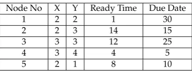
Table2includes all the relevant data of the above example. In particular, we see the coordinates X 268

and Y of every node, as well as the Ready Time and the Due Date. 269

Table 2.The input data for our example.

Node No X Y Ready Time Due Date

1 2 2 1 30

2 2 3 14 15

3 3 3 12 25

4 3 4 4 5

5 2 1 8 10

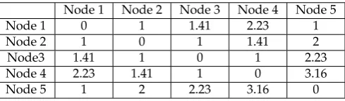
Table3is actually the distance matrix for our example. Let us clarify here that we calculated 270

the costs between the nodes using the Euclidean distance, which is given by the well-know formula: 271

Table 3.The distance matrix.

Node 1 Node 2 Node 3 Node 4 Node 5

Node 1 0 1 1.41 2.23 1

Node 2 1 0 1 1.41 2

Node3 1.41 1 0 1 2.23

Node 4 2.23 1.41 1 0 3.16

Node 5 1 2 2.23 3.16 0

A feasible solution for this particular TSPTW consisting of 5 nodes is given in Table4. One can 273

see that if all time windows are respected in every step of the tour going from from one customer to 274

the next, a feasible solution can be constructed. Although, this is a small scale example, we expect that 275

it will enhance one’s understanding of what is a feasible solution for the TSPTW. 276

Table 4.A feasible solution of our illustrated example.

Ordering Node 1 Node 4 Node 5 Node 3 Node 2

cost 0<1 2.23 <4 7.16 <8 10 <12 12<14

feasibility yes yes yes yes yes

In the next section we introduce our novel approach for mapping the TSPTW over the quadratic 277

unconstrained binary optimization (QUBO) model. 278

4. A QUBO formulation for the TSPTW 279

In the literature, the typical QUBO formulation of the standard TSP involves the use of a set of 280

binaryvariables (see [32]). They are characterized as binary in the sense that they can take only the 0 or 281

1 value. Typically, they are denoted byxv,i, and their meaning is the following: 282

xv,i = (

1, customervis at positioniin the tour

0, otherwise . (5)

In the case of the TSPTW, we have discovered to be more advantageous to use binary variables 283

parameterized by three integers: u,vandi. A similar suggestion for the Vehicle Routing Problem can 284

be found in [38]. Hence, in the rest of our analysis, we shall use the binary variablesxiu,vdefined next: 285

xiu,v= (

1, customersuandvare at consecutive positionsi−1 andiin the tour

0, otherwise . (6)

As we explained in the previous section, a feasible tour has the form{p0,p1, . . . ,pn,pn+1}. In 286

this enumeration,piis the customer in theithposition of the tour. We always take for granted that 287

p0= pn+1=0 and each other customer appears exactly once. We recall the assumption ofzero service 288

timeat each customer, and without loss of generality, we adopt another assumption that greatly reduces 289

the final clutter of our QUBO expressions: for each customerv, where 0≤v≤n+1,ev=0. With this 290

understanding, we see that the parametersuandvrange from 0 tonand the parameteriranges from 291

1 ton+1. 292

Therefore, we can assert that: 293

• For eachi, 1≤i≤n+1, exactly one of the binary variablesxui,vis 1, whereuandvrange freely 294

from 0 ton, with the proviso thatu 6=v. As a matter of fact wheni=1 andi=n+1 we can 295

be more precise. In the former case, exactly one of the binary variablesx1

0,vis 1, wherevranges 296

from 1 ton, and, in the latter case, exactly one of the binary variablesxn_v,0+1is 1, wherevranges 297

• In addition to the above constraints, for eachu, 1≤u≤n, exactly one of the binary variables 299

xi_u,vis 1, whereiranges from 2 tonandvranges from 1 ton. 300

• Symmetrically, we also have the constraint that for everyv, 1≤v≤n, exactly one of the binary 301

variablesx_ui_,vis 1, whereiranges from 2 tonanduranges from 1 ton. 302

These constraints are encoded in the HamiltonianHc. 303

Hc=B n+1

∑





1−

n

∑

n

∑

xiu,v 

  2

+B 1− n

∑

x0,1v

!2

+B 1− n

∑

xn_v+_,01

!2

+B n

∑

1− n

∑

n

∑

xiu,v

!2

(7)

+B n

∑

1− n

∑

n

∑

xiu,v

!2

Using thexi_u,vbinary variables, the requirement that the tour be minimal can be encoded by the 304

following HamiltonianHm. 305

Hm=C n+1

∑

n

∑

n

∑

xiu,vcu,v. (8)

In the above Hamiltonians,BandCare positive constants, which must be appropriately chosen, 306

i.e.,C<B, so as to ensure that the constraints ofHcare respected (see also [32]). Obviously,cu,vis the 307

cost for traversing the arc(u,v). 308

The above Hamiltonians are certainly not the end of the story in the case of the TSPTW, as, in their 309

essence, they just encode the minimal cost of the Hamiltonian circuit. There are a lot more difficult 310

time constraints to tackle in order to satisfy the time window of every customer. To this end, besides 311

the binary variablesxi

u,v, it will be necessary to use a second type of binary variables, denoted bytn,i, 312

in order to express thetime marginof every customer. 313

Definition 5. Given afeasibletour p0,p1, . . . ,pn,pn+1, suppose that the customer at position i, where 314

1≤ i ≤ n, is v with time window[ev,lv]. We say that thetime marginof the customer at position i to be 315

lv−Ap_i. 316

Clearly, for a feasible tour, the time margin for every position of the tour is non negative. We can 317

now define the binary variablestk,ias follows: 318

tk,i= (

1, the time margin of the customer at positioniin the tour isk

0, otherwise . (9)

We recall that in the formulation of the TSPTW, the arrival time at the customer in theithposition 319

of the tour, denotedAp_i, plays an important role (see [73]). Thus, we begin our analysis by showing 320

how to expressAp_i. Obviously,Ap₀ =0, so it is only necessary to give the formula forAp_i, 1≤i≤n. 321

We first observe that the customer at position 0 is always the depot (customer 0), which results in the 322

following, relatively simple formula, forAp₁. 323

Ap₁ = n

∑

x10,vc0,v. (10)

Ap_i = i

∑

n

∑

n

∑

xdu,vcu,v (2≤i≤n). (11)

Example 1. To explain how Equations (10) and (11) can be used in practice, we continue with our test case 325

example. 326

Equation (10) becomes 327

Ap₁ =x1_0,1c0,1+x10,2c0,2+x10,3c0,3+x10,4c0,4 (12) Equation (11) gives the following series of equations.

328

Ap₂ = 

  

x1_0,1c0,1+x10,2c0,2+x10,3c0,3+x10,4c0,4

| {z }

Ap₁



  

+x2_1,2c1,2+x1,32 c1,3+x1,42 c1,4+x22,1c2,1+x22,3c2,3+x22,4c2,4 (13) +x2_3,1c3,1+x3,22 c3,2+x3,42 c3,4+x24,1c4,1+x4,22 c4,2+x24,3c4,3

Ap₃ =

x_0,11 c0,1+x10,2c0,2+x10,3c0,3+x10,4c0,4

+x2_1,2c1,2+x1,32 c1,3+x21,4c1,4+x2,12 c2,1+x2,32 c2,3+x22,4c2,4 +x23,1c3,1+x3,22 c3,2+x23,4c3,4+x4,12 c4,1+x4,22 c4,2+x24,3c4,3

(14)

+x3_1,2c1,2+x1,33 c1,3+x31,4c1,4+x2,13 c2,1+x2,33 c2,3+x32,4c2,4 +x3_3,1c3,1+x3,23 c3,2+x33,4c3,4+x4,13 c4,1+x4,23 c4,2+x34,3c4,3

Ap₄ =x1_0,1c0,1+x10,2c0,2+x0,31 c0,3+x10,4c0,4

+x2_1,2c1,2+x1,32 c1,3+x1,42 c1,4+x22,1c2,1+x2,32 c2,3+x22,4c2,4 +x2_3,1c3,1+x3,22 c3,2+x3,42 c3,4+x24,1c4,1+x4,22 c4,2+x24,3c4,3

+x3_1,2c1,2+x1,33 c1,3+x1,43 c1,4+x32,1c2,1+x32,3c2,3+x32,4c2,4 (15) +x3_3,1c3,1+x3,23 c3,2+x3,43 c3,4+x34,1c4,1+x4,23 c4,2+x34,3c4,3

+x4_1,2c1,2+x1,34 c1,3+x1,44 c1,4+x42,1c2,1+x2,34 c2,3+x42,4c2,4 +x4_3,1c3,1+x3,24 c3,2+x3,44 c3,4+x44,1c4,1+x4,24 c4,2+x44,3c4,3

The above equations demonstrate that in every case, Ap_ican be expressed as a sum of terms, where each 329

term is the product of an input variable cu,vandexactly onebinary decision variable xui,v. 330

The simplifying assumption of zero service time enables us to express the constraints imposed by 331

the time windows of every customer as follows: 332

Ap₁ ≤ n

∑

for the special case wherei=1, and

Ap_i ≤ n

∑

n

∑

xiu,vlv (2≤i≤n), (17)

for the general case where 2≤i≤n. 333

The above expression may seem a little complicated, but, unfortunately, whileAp_i tells us the 334

arrival time at the customer in theithposition of the tour, it does not tell uswhich isthis particular 335

customer. We have to resort to the binary variablesxi_u,vto indirectly obtain this information. 336

Inequality constraints such as these in (16) and (17) are notoriously difficult to express within the 337

QUBO framework. For an extensive analysis we refer the interested reader to [28,59,74]. The approach 338

which is most commonly used in the literature is to employ auxiliary binary variables, like the binary 339

variablestk,ipreviously defined, to convert the inequality into an equality, and then proceed, as usual, 340

by squaring the equality constraint. 341

In our case, the first step is to express the inequalities (16) and (17) as 342

Ap₁+ K

∑

ktk,1= n

∑

x1_0,vlv, (18)

and as

Ap_i+ K

∑

ktk,i = n

∑

n

∑

xiu,vlv (2≤i≤n), (19)

respectively. 343

In the above equalitiesKis a positive constant appropriately chosen taking into consideration 344

the specific time windows. A valid possible choice could beK=max1≤v≤n{lv}. Such a choice, while 345

valid, would be unnecessarily big in most practical cases. 346

Equality constraints like (18) and (19) are typically treated in QUBO by converting them into 347

squared expressions. Hence, (18) gives rise to the first time window constraint, denoted byW1and 348

given by 349

W1= Ap1+ K

∑

ktk,i− n

∑

x10,vlv

!2

, (20)

while Equation (19) gives rise to theith_{time window constraint, denoted byW}

iand given by:

Wi = 



Api+

K

∑

ktk,i− n

∑

n

∑

xi_u,vlv 

  2

(2≤i≤n). (21)

If we replaceAp₁and Ap_i in the above equations by the formulas in (10) and (11), we derive the 350

expanded forms ofW1andWi, 2≤i≤n, respectively. 351

W1= n

∑

x10,vc0,v+ K

∑

ktk,i− n

∑

x10,vlv

!2

Wi= 

  i

∑

n

∑

n

∑

xdu,vcu,v+ K

∑

ktk,i− n

∑

n

∑

xiu,vlv 

  2

(2≤i≤n). (23)

At this point it is important to pause and confirm that the constraints in Equations (22) and (23) 352

conform to the QUBO formulation requirements, in the sense that, after the expansion of the square, 353

we get a sum of terms, where each term is the product of input data likecu,vorlv andat most two 354

binary decision variables. 355

The last time constraint concerns the binary variablestk,i. For eachi, 1≤i≤n, exactly one of 356

the binary variablestk,iis 1, wherekranges from 1 toK. The meaning of this constraint is obvious: in 357

every position of a feasible tour the time margin should be unique. Expressing this constraint is also 358

straightforward: 359

Mi= 1− K

∑

tk,i

!2

(1≤i≤n). (24)

Putting all the time constraints together results in the HamiltonianHt: 360

Ht=T(W1) +T n

∑

TWCi+T n

∑

Mi. (25)

Therefore, to solve the TSPTW in the QUBO framework we must use the HamiltonianHgiven 361

below: 362

H= Hc+Hm+Ht. (26)

As noted earlier, the constantsB,CandTappearing in the Hamiltonians are positive constants, 363

which must be chosen according to our requirements. For instance, by settingC < B, so as to 364

ensure that the constraints ofHcare respected; similarly, settingT<Bprioritizes the time windows 365

constraints over the minimality of the tour. 366

Example 2. To show the form of the time windows constraints when the square is expanded, we apply 367

constraint (22) to our test case example. 368

First we point out that for binary variables the following hold: 369

(xi_u,v)2=xi_u,v and (tk,i)2=tk,i. (27) We also recall the identity:(a+b−c)2=a2+b2+c2+2ab−2ac−2bc. We shall use this identity to 370

expand (22), setting a =_∑n_v=1x1_0,vc0,v, b=∑Kk=1ktk,1, and c=∑nv=1x10,vlv. In our example n=4and, in 371

order to simplify somewhat the calculations we take K=2. With this understanding we use Equation (12) to 372

derive the formulas given below. Note that to improve the readability of the equations in this example, we have 373

written in green color those terms that involveexactly onebinary variable and in blue color those terms that 374

A2p1 =

x1_0,1c0,1+x10,2c0,2+x10,3c0,3+x0,41 c0,4

2

= (x1_0,1)2c2_0,1+ (x10,2)2c20,2+ (x10,3)2c20,3+ (x0,41 )2c20,4+2x10,1c0,1x0,21 c0,2+2x10,1c0,1x10,3c0,3 +2x10,1c0,1x0,41 c0,4+2x10,2c0,2x10,3c0,3+2x10,2c0,2x10,4c0,4+2x10,3c0,3x0,41 c0,4 (28) =x1_0,1c2_0,1+x1_0,2c_0,22 +x1_0,3c2_0,3+x1_0,4c2_0,4+2x1_0,1c0,1x0,21 c0,2+2x10,1c0,1x10,3c0,3

+2x1_0,1c0,1x_0,41 c0,4+2x1_0,2c0,2x1_0,3c0,3+2x1_0,2c0,2x1_0,4c0,4+2x1_0,3c0,3x_0,41 c0,4

Similarly, we see that: 376

2

∑

ktk,1

!2

= (1t1,1+2t2,1)2=t21,1+4t22,1+4t1,1t2,1=t1,1+4t2,1+4t1,1t2,1 (29)

4

∑

x1_0,vlv

!2

= x1_0,1l1+x10,2l2+x10,3l3+x10,4l4

2

= (x1_0,1)2l₁2+ (x1_0,2)2l₂2+ (x1_0,3)2l₃2+ (x_0,41 )2l₄2+2x1_0,1l1x0,21 l2+2x10,1l1x10,3l3 +2x1_0,1l1x10,4l4+2x10,2l2x10,3l3+2x0,21 l2x0,41 l4+2x10,3l3x10,4l4 (30) =x1_0,1l₁2+x10,2l22+x10,3l23+x10,4l42+2x10,1l1x0,21 l2+2x10,1l1x10,3l3

+2x1_0,1l1x10,4l4+2x10,2l2x10,3l3+2x0,21 l2x0,41 l4+2x10,3l3x10,4l4

2Ap₁ 2

∑

ktk,1=2

x1_0,1c0,1+x10,2c0,2+x10,3c0,3+x10,4c0,4

(1t1,1+2t2,1)

=2x10,1c0,1t1,1+2x10,1c0,1t2,1+2x10,2c0,2t1,1+2x10,2c0,2t2,1 (31)

+2x1_0,3c0,3t1,1+2x10,3c0,3t2,1+2x10,4c0,4t1,1+2x10,4c0,4t2,1

2Ap₁ 4

∑

x1_0,vlv=2x1_0,1c0,1+x10,2c0,2+x10,3c0,3+x10,4c0,4 x10,1l1+x10,2l2+x10,3l3+x10,4l4

=2(x_0,11 )2c0,1l1+2x0,11 c0,1x10,2l2+2x10,1c0,1x10,3l3+2x10,1c0,1x10,4l4 +2x1_0,2c0,2x10,1l1+2(x10,2)2c0,2l2+2x10,2c0,2x10,3l3+2x10,2c0,2x10,4l4 +2x1_0,3c0,3x10,1l1+2x10,3c0,3x10,2l2+2(x10,3)2c0,3l3+2x10,3c0,3x10,4l4 +2x10,4c0,4x10,1l1+2x10,4c0,4x10,2l2+2x10,4c0,4x10,3l3+2(x10,4)2c0,4l4

=2x1_0,1c0,1l1+2x10,2c0,2l2+2x10,3c0,3l3+2x10,4c0,4l4 (32)

+2x1_0,1c0,1x1_0,2l2+2x_0,11 c0,1x1_0,3l3+2x1_0,1c0,1x1_0,4l4

+2x10,2c0,2x10,1l1+2x0,21 c0,2x10,3l3+2x10,2c0,2x10,4l4

+2x10,3c0,3x10,1l1+2x0,31 c0,3x10,2l2+2x10,3c0,3x10,4l4

2

2

∑

ktk,1 4

∑

x1_0,vlv=2(1t1,1+2t2,1)

x1_0,1l1+x10,2l2+x10,3l3+x10,4l4

=2t1,1x10,1l1+2t1,1x10,2l2+2t1,1x10,3l3+2t1,1x10,4l4 (33)

+4t2,1x1_0,1l1+4t2,1x1_0,2l2+4t2,1x1_0,3l3+4t2,1x1_0,4l4

We can now substitute Equations (28)–(33) in (22) to finally arrive at the expanded form of the constraint, 377

given by the following equation. 378

W1=x10,1c20,1+x0,21 c20,2+x10,3c20,3+x10,4c20,4+2x10,1c0,1x0,21 c0,2+2x10,1c0,1x10,3c0,3 +2x1_0,1c0,1x10,4c0,4+2x10,2c0,2x10,3c0,3+2x0,21 c0,2x10,4c0,4+2x10,3c0,3x10,4c0,4

+t1,1+4t2,1+4t1,1t2,1

+x1_0,1l₁2+x_0,21 l2₂+x1_0,3l2₃+x1_0,4l₄2+2x1_0,1l1x_0,21 l2+2x1_0,1l1x1_0,3l3

+2x1_0,1l1x1_0,4l4+2x10,2l2x10,3l3+2x0,21 l2x10,4l4+2x10,3l3x10,4l4

−2x1_0,1c0,1t1,1−2x10,1c0,1t2,1−2x10,2c0,2t1,1−2x10,2c0,2t2,1 −2x1_0,3c0,3t1,1−2x10,3c0,3t2,1−2x10,4c0,4t1,1−2x10,4c0,4t2,1

−2x1_0,1c0,1l1−2x10,2c0,2l2−2x10,3c0,3l3−2x0,41 c0,4l4 (34)

−2x1_0,1c0,1x10,2l2−2x0,11 c0,1x10,3l3−2x0,11 c0,1x10,4l4

−2x1_0,2c0,2x0,11 l1−2x10,2c0,2x0,31 l3−2x0,21 c0,2x10,4l4 −2x1_0,3c0,3x1_0,1l1−2x0,31 c0,3x10,2l2−2x0,31 c0,3x10,4l4

−2x1_0,4c0,4x1_0,1l1−2x_0,41 c0,4x1_0,2l2−2x_0,41 c0,4x1_0,3l3

−2t1,1x_0,11 l1−2t1,1x0,21 l2−2t1,1x0,31 l3−2t1,1x0,41 l4

−4t2,1x0,11 l1−4t2,1x0,21 l2−4t2,1x0,31 l3−4t2,1x0,41 l4

Similar calculations, albeit too lengthy to include here, confirm that all time window constraints have 379

similar patterns, that is they constitute legitimate expressions within the QUBO framework. 380

5. Conclusions and future work 381

In this work, we have considered the TSPTW. Although many combinatorial optimization 382

problems have been expressed in the QUBO (or, equivalently, the Ising) formulation, this particular 383

problem was not one of them. Presumably, the reason is the TSPTW imposes many additional (time) 384

constraints because the customers’ time windows must be satisfied. These are actually inequality 385

constraints that are very difficult to tackle within the QUBO framework. We remind the reader that 386

valid QUBO expressions must have the form: xTQx, wherexis a column vector of binary decision 387

variables,xT_{its transpose andQa square matrix of constants. So, to the best of our knowledge, this is} 388

the first time the TSPTW is cast in QUBO form. 389

This step is a necessary precondition in order to be able to run TSPTW instances on the current 390

generation of D-Wave computers. Hence, the future direction of this work will the mapping of TSPTW 391

benchmarks to the Chimera or the upcoming Pegasus architecture, so as to obtain experimental results. 392

This will enable the comparison of the current state of the art classical, or conventional, if you prefer, 393

metaheuristics with the purely quantum approach. This comparison is expected to shed some light on 394

the pressing question of whether quantum annealing is more efficient than classical methods, and, if 395

so, to what degree. 396

Author Contributions: Conceptualization, Christos Papalitsas and Theodore Andronikos; Formal

397

analysis,Christos Papalitsas and Theodore Andronikos; Methodology, Christos Papalitsas and Theodore

Andronikos; Supervision, Theodore Andronikos; Validation, Christos Papalitsas and Sofia Fanarioti; Writing

-399

original draft, Konstantinos Giannakis and Georgia Theocharopoulou; Writing - review & editing, Konstantinos

400

Giannakis, Georgia Theocharopoulou, Christos Papalitsas, Sofia Fanarioti and Theodore Andronikos.

401

Funding:This research is funded in the context of the project “Investigating alternative computational methods

402

and their use in computational problems related to optimization and game theory,” (MIS 5007500) under the

403

call for proposals “Supporting researchers with an emphasis on young researchers” (EDULL34). The project is

404

co-financed by Greece and the European Union (European Social Fund - ESF) by the Operational Programme

405

Human Resources Development, Education and Lifelong Learning 2014-2020.

406

Conflicts of Interest:The authors declare no conflicts of interest.

407

Abbreviations 408

The following abbreviations are used in this manuscript:

409 410

QPU Quantum Processing Unit

QUBO Quadratic Unconstrained Binary Optimization

TSP Traveling Salesman Problem

TSPTW Traveling Salesman Problem with Time Windows

411

412

1. Feynman, R.P. Simulating physics with computers. International Journal of Theoretical Physics Int J Theor 413

Phys1982,21, 467–488.

414

2. Shor, P.W. Polynomial-time algorithms for prime factorization and discrete logarithms on a quantum

415

computer. SIAM review1999,41, 303–332.

416

3. Grover, L. A fast quantum mechanical algorithm for database search. Proc. of the Twenty-Eighth Annual

417

ACM Symposium on the Theory of Computing, 1996, 1996.

418

4. Nielsen, M.A.; Chuang, I.L.Quantum computation and quantum information; Cambridge university press,

419

2010.

420

5. Farhi, E.; Goldstone, J.; Gutmann, S.; Sipser, M. Quantum computation by adiabatic evolution. arXiv 421

preprint quant-ph/00011062000.

422

6. Farhi, E.; Goldstone, J.; Gutmann, S.; Lapan, J.; Lundgren, A.; Preda, D. A quantum adiabatic evolution

423

algorithm applied to random instances of an NP-complete problem.Science2001,292, 472–475.

424

7. Choi, V. Minor-embedding in adiabatic quantum computation: I. The parameter setting problem.Quantum 425

Information Processing2008,7, 193–209.

426

8. Messiah, A. Quantum mechanics, 1961.

427

9. Amin, M. Consistency of the adiabatic theorem.Physical review letters2009,102, 220401.

428

10. Kadowaki, T. Study of optimization problems by quantum annealing. arXiv preprint quant-ph/0205020 429

2002.

430

11. Kadowaki, T.; Nishimori, H. Quantum annealing in the transverse Ising model. Physical Review E1998,

431

58, 5355.

432

12. Kirkpatrick, S.; Gelatt, C.D.; Vecchi, M.P. Optimization by simulated annealing.science1983,220, 671–680.

433

13. Pakin, S. Performing fully parallel constraint logic programming on a quantum annealer. Theory and 434

Practice of Logic Programming2018,18, 928–949.

435

14. Perdomo-Ortiz, A.; Dickson, N.; Drew-Brook, M.; Rose, G.; Aspuru-Guzik, A. Finding low-energy

436

conformations of lattice protein models by quantum annealing. Scientific reports2012,2, 571.

437

15. Sarkar, A. Quantum Algorithms: for pattern-matching in genomic sequences2018.

438

16. Biamonte, J.; Wittek, P.; Pancotti, N.; Rebentrost, P.; Wiebe, N.; Lloyd, S. Quantum machine learning.

439

Nature2017,549, 195.

440

17. Papalitsas, C.; Karakostas, P.; Andronikos, T.; Sioutas, S.; Giannakis, K. Combinatorial GVNS (General

441

Variable Neighborhood Search) Optimization for Dynamic Garbage Collection.Algorithms2018,11, 38.

442

18. Rebentrost, P.; Schuld, M.; Wossnig, L.; Petruccione, F.; Lloyd, S. Quantum gradient descent and Newton’s

443

method for constrained polynomial optimization.New Journal of Physics2019.

444

19. D-Wave, S. Getting Started with the D-Wave System. Technical report, D-Wave Systems, 2019.

20. Boothby, K.; Bunyk, P.; Raymond, J.; Roy, A. Next-generation topology of D-Wave quantum processors.

446

Technical report, D-Wave Systems, 2019.

447

21. Dattani, N.; Szalay, S.; Chancellor, N. Pegasus: The second connectivity graph for large-scale quantum

448

annealing hardware.arXiv preprint arXiv:1901.076362019.

449

22. Dattani, N.; Chancellor, N. Embedding quadratization gadgets on Chimera and Pegasus graphs. arXiv 450

preprint arXiv:1901.076762019.

451

23. Boros, E.; Crama, Y.; Hammer, P.L. Upper-bounds for quadratic 0–1 maximization. Operations Research 452

Letters1990,9, 73–79.

453

24. Lewis, M.; Glover, F. Quadratic unconstrained binary optimization problem preprocessing: Theory and

454

empirical analysis. Networks2017,70, 79–97.

455

25. Kochenberger, G.; Hao, J.K.; Glover, F.; Lewis, M.; Lü, Z.; Wang, H.; Wang, Y. The unconstrained binary

456

quadratic programming problem: a survey.Journal of Combinatorial Optimization2014,28, 58–81.

457

26. Lloyd, S.; Mohseni, M.; Rebentrost, P. Quantum algorithms for supervised and unsupervised machine

458

learning.arXiv preprint arXiv:1307.04112013.

459

27. Hauke, P.; Katzgraber, H.G.; Lechner, W.; Nishimori, H.; Oliver, W.D. Perspectives of quantum annealing:

460

Methods and implementations. arXiv preprint arXiv:1903.065592019.

461

28. Glover, F.; Kochenberger, G. A Tutorial on Formulating QUBO Models. arXiv preprint arXiv:1811.11538 462

2018.

463

29. Boros, E.; Hammer, P.L.; Tavares, G. Local search heuristics for quadratic unconstrained binary optimization

464

(QUBO).Journal of Heuristics2007,13, 99–132.

465

30. Ushijima-Mwesigwa, H.; Negre, C.F.; Mniszewski, S.M. Graph partitioning using quantum annealing

466

on the D-Wave system. Proceedings of the Second International Workshop on Post Moores Era

467

Supercomputing. ACM, 2017, pp. 22–29.

468

31. Newell, G.F.; Montroll, E.W. On the theory of the Ising model of ferromagnetism.Reviews of Modern Physics 469

1953,25, 353.

470

32. Lucas, A. Ising formulations of many NP problems.Frontiers in Physics2014,2, 5.

471

33. Neukart, F.; Compostella, G.; Seidel, C.; Von Dollen, D.; Yarkoni, S.; Parney, B. Traffic flow optimization

472

using a quantum annealer. Frontiers in ICT2017,4, 29.

473

34. Marto ˇnák, R.; Santoro, G.E.; Tosatti, E. Quantum annealing of the traveling-salesman problem. Physical 474

Review E2004,70, 057701.

475

35. Warren, R.H. Adapting the traveling salesman problem to an adiabatic quantum computer. Quantum 476

information processing2013,12, 1781–1785.

477

36. Warren, R.H. Small traveling salesman problems. Journal of Advances in Applied Mathematics2017,2.

478

37. Feld, S.; Roch, C.; Gabor, T.; Seidel, C.; Neukart, F.; Galter, I.; Mauerer, W.; Linnhoff-Popien, C. A hybrid

479

solution method for the capacitated vehicle routing problem using a quantum annealer. arXiv preprint 480

arXiv:1811.074032018.

481

38. Irie, H.; Wongpaisarnsin, G.; Terabe, M.; Miki, A.; Taguchi, S. Quantum annealing of vehicle routing

482

problem with time, state and capacity. International Workshop on Quantum Technology and Optimization

483

Problems. Springer, 2019, pp. 145–156.

484

39. Neven, H.; Denchev, V.S.; Rose, G.; Macready, W.G. Training a large scale classifier with the quantum

485

adiabatic algorithm.arXiv preprint arXiv:0912.07792009.

486

40. Garnerone, S.; Zanardi, P.; Lidar, D.A. Adiabatic quantum algorithm for search engine ranking. Physical 487

review letters2012,108, 230506.

488

41. Cruz-Santos, W.; Venegas-Andraca, S.; Lanzagorta, M. A QUBO Formulation of the Stereo Matching

489

Problem for D-Wave Quantum Annealers. Entropy2018,20, 786.

490

42. Babbush, R.; Love, P.J.; Aspuru-Guzik, A. Adiabatic quantum simulation of quantum chemistry.Scientific 491

reports2014,4, 6603.

492

43. Crispin, A.; Syrichas, A. Quantum annealing algorithm for vehicle scheduling. 2013 IEEE International

493

Conference on Systems, Man, and Cybernetics. IEEE, 2013, pp. 3523–3528.

494

44. Cai, B.B.; Zhang, X.H. Hybrid Quantum Genetic Algorithm and Its Application in VRP [J]. Computer 495

Simulation2010,7.

496

45. Binder, K.; Young, A.; Fischer, K.; Hertz, J. Rev. Mod. Phys., 1986.

497

46. Young, A.P.Spin glasses and random fields; Vol. 12, World Scientific, 1998.

47. Nishimori, H. Statistical physics of spin glasses and information processing: an introduction; Number 111,

499

Clarendon Press, 2001.

500

48. Venturelli, D.; Mandra, S.; Knysh, S.; O’Gorman, B.; Biswas, R.; Smelyanskiy, V. Quantum optimization of

501

fully connected spin glasses. Physical Review X2015,5, 031040.

502

49. Titiloye, O.; Crispin, A. Quantum annealing of the graph coloring problem. Discrete Optimization2011,

503

8, 376–384.

504

50. Venturelli, D.; Marchand, D.J.; Rojo, G. Quantum annealing implementation of job-shop scheduling.arXiv 505

preprint arXiv:1506.084792015.

506

51. Benedetti, M.; Realpe-Gómez, J.; Biswas, R.; Perdomo-Ortiz, A. Quantum-assisted learning of

507

hardware-embedded probabilistic graphical models.Physical Review X2017,7, 041052.

508

52. Battaglia, D.A.; Santoro, G.E.; Tosatti, E. Optimization by quantum annealing: Lessons from hard

509

satisfiability problems. Physical Review E2005,71, 066707.

510

53. Alom, M.Z.; Van Essen, B.; Moody, A.T.; Widemann, D.P.; Taha, T.M. Quadratic Unconstrained Binary

511

Optimization (QUBO) on neuromorphic computing system. 2017 International Joint Conference on Neural

512

Networks (IJCNN). IEEE, 2017, pp. 3922–3929.

513

54. Pagano, G.; Bapat, A.; Becker, P.; Collins, K.; De, A.; Hess, P.; Kaplan, H.; Kyprianidis, A.; Tan, W.; Baldwin,

514

C.; others. Quantum Approximate Optimization with a Trapped-Ion Quantum Simulator.arXiv preprint 515

arXiv:1906.027002019.

516

55. Farhi, E.; Harrow, A.W. Quantum supremacy through the quantum approximate optimization algorithm.

517

arXiv preprint arXiv:1602.076742016.

518

56. Venegas-Andraca, S.E.; Cruz-Santos, W.; McGeoch, C.; Lanzagorta, M. A cross-disciplinary introduction to

519

quantum annealing-based algorithms.Contemporary Physics2018,59, 174–197.

520

57. Farhi, E.; Goldstone, J.; Gutmann, S. A quantum approximate optimization algorithm. arXiv preprint 521

arXiv:1411.40282014.

522

58. Hadfield, S.; Wang, Z.; O’Gorman, B.; Rieffel, E.G.; Venturelli, D.; Biswas, R. From the quantum

523

approximate optimization algorithm to a quantum alternating operator ansatz. Algorithms2019,12, 34.

524

59. Vyskocil, T.; Djidjev, H. Embedding Equality Constraints of Optimization Problems into a Quantum

525

Annealer.Algorithms2019,12. doi:10.3390/a12040077.

526

60. Barán, B.; Villagra, M. A Quantum Adiabatic Algorithm for Multiobjective Combinatorial Optimization.

527

Axioms2019,8, 32.

528

61. Oliveira, N.M.D.; Silva, R.M.D.A.; Oliveira, W.R.D. QUBO formulation for the contact map overlap

529

problem.International Journal of Quantum Information2018,16, 1840007.

530

62. Rosenberg, G.; Vazifeh, M.; Woods, B.; Haber, E. Building an iterative heuristic solver for a quantum

531

annealer.Computational Optimization and Applications2016,65, 845–869.

532

63. Langevin, A.; Desrochers, M.; Desrosiers, J.; Gélinas, S.; Soumis, F. A two-commodity flow formulation for

533

the traveling salesman and the makespan problems with time windows. Networks1993,23, 631–640.

534

64. Dumas, Y.; Desrosiers, J.; Gelinas, E.; Solomon, M.M. An optimal algorithm for the traveling salesman

535

problem with time windows.Operations research1995,43, 367–371.

536

65. Gendreau, M.; Hertz, A.; Laporte, G.; Stan, M. A generalized insertion heuristic for the traveling salesman

537

problem with time windows.Operations Research1998,46, 330–335.

538

66. Da Silva, R.F.; Urrutia, S. A General VNS heuristic for the traveling salesman problem with time windows.

539

Discrete Optimization2010,7, 203–211.

540

67. Sotiropoulos, D.; Stavropoulos, E.; Vrahatis, M. A new hybrid genetic algorithm for global optimization.

541

Nonlinear Analysis: Theory, Methods & Applications1997,30, 4529–4538.

542

68. Pardalos, P.M.; Rodgers, G.P. Computational aspects of a branch and bound algorithm for quadratic

543

zero-one programming. Computing1990,45, 131–144.

544

69. Lahoz-Beltra, R. Quantum genetic algorithms for computer scientists.Computers2016,5, 24.

545

70. Papalitsas, Ch.; Giannakis, K.; Andronikos, Th.; Theotokis, D.; Sifaleras, A. Initialization methods for

546

the TSP with Time Windows using Variable Neighborhood Search. IEEE Proc. of the 6th International

547

Conference on Information, Intelligence, Systems and Applications (IISA 2015), 6-8 July, Corfu, Greece,

548

2015.

549

71. Papalitsas, C.; Karakostas, P.; Kastampolidou, K. A Quantum Inspired GVNS: Some Preliminary Results.

550

GeNeDis 2016; Vlamos, P., Ed.; Springer International Publishing: Cham, 2017; pp. 281–289.

72. Papalitsas, C.; Andronikos, T. Unconventional GVNS for Solving the Garbage Collection Problem with

552

Time Windows. Technologies2019,7. doi:10.3390/technologies7030061.

553

73. Ohlmann, J.W.; Thomas, B.W. A compressed-annealing heuristic for the traveling salesman problem with

554

time windows.INFORMS Journal on Computing2007,19, 80–90.

555

74. Vyskoˇcil, T.; Pakin, S.; Djidjev, H.N. Embedding Inequality Constraints for Quantum Annealing

556

Optimization. Quantum Technology and Optimization Problems; Feld, S.; Linnhoff-Popien, C., Eds.;

557

Springer International Publishing: Cham, 2019; pp. 11–22.