IJEDR1603067
International Journal of Engineering Development and Research (www.ijedr.org)415
Optimal Design of Low Pass Digital FIR Filter Using
Soft Computational Technique
1Navneet Kaur, 2Balraj Singh
1M.tech (Scholar), 2Associate Professor (ECE) 1Department of Electronics and Communication Engineering,
1Gaini Zail Singh Campus College of Engineering and Technology, Bathinda-151001, Punjab, India
Abstract- The objective of this paper elaborates a procedure for designing of low pass digital finite impulse response filter
with the use of Predator-Prey Optimization method. Predator-Prey Optimization (PPO) is stochastic optimization technique where the predator explores for global best in a robust manner and preys search for solution space owing to predator fear. Predator helps to avoid incomplete convergence in local optima. Various parameters like population size, acceleration constants have been tuned to attain better results.
Key Words- Digital FIR filters, Predator Prey Optimization, Low pass filter, Magnitude response and phase response.
I. INTRODUCTION
Signal is bulk of information which is transmissible and it modifies with space and time. Processing is a chain of operations to attain a particular conclusion. So, signal processing is any physical or mechanical process that modifies or manipulates information that is enclosed in the signal. So, “Digital signal processing” is the mathematical handling of signals, with the aim of filtering, compressing, evaluating and processing analog signals. DSP have various applications in sectors of image processing, telecommunication, speech processing, biomedical and in huge range of other applications [8].
Filter being a part of a signal processing, is an electrical circuit that eliminates unwanted portion of the signal present at its output [4]. This means, it is the process of eliminating some frequencies in command to suppress the intrusive signals and diminish background noise. Based upon the selection of frequencies, filters can be categorized as Low-pass, High-pass, Band-pass and Band-stop filters. Basically filters are of two types named- analog filter and digital filter. Analog filter works on analog signals which are continuous in nature like Bessel filter, Chebyshev filter, Gaussian filter, etc, whereas digital filters perform numerical operations on sampled, discrete-time signals to decrease or improve certain forms of the signals. Digital filters serves two functions firstly, used for signal separation when signal is contaminated with the noise and secondly, for the restoration of signals when it has been distorted along the transmission path. Further digital filters are classified as infinite impulse response (IIR) and finite impulse response (FIR) filters. IIR filters are called recursive filters because the output is fedback to the input side and FIR filters are termed as non-recursive due to the absence of feedback. The advantages of FIR filter over IIR filter are stability, linear phase and easy control. In addition, the output of FIR depends only on the input. Apart from these advantages, FIR filter requires large amount of memory, filter coefficients and computational time as compared to IIR filter [11].
The methods for the design of FIR filter are Window method, Frequency Sampling method and Optimization method [6]. Window method is simple and easy to use but it lacks in contributing sufficient flexibility [5]. Frequency sampling technique is used for designing filters by specifying the magnitude response of filter. Though, the desired frequency response is equivalent to the obtained frequency response only at the sampled values. Optimization is described as maximization or minimization of a function. To improve the robustness of the filter, various optimization design techniques have been applied like particle swarm optimization (PSO), differential evolution (DE), genetic algorithm, etc [11]. DE is simple, easy to use and population based optimization algorithm [9]. PSO converges very rapidly as compared to other techniques, but due to wrong choices of initial parameters, it may get trap in local minima. PPO is more valuable as predator effect is carried along with population based technique (PSO) [7].
This paper has five sections. Section 2 depicts Design Formulation. Section 3 focuses on PPO algorithm. The performance and results have been explained in the Section 4. Section 5 covers conclusion.
II. DESIGN FORMULATION
FIR Filter does not require any feedback from the output side, thus entitled as non-recursive filters [8]. Because of its property of linear phase, FIR Filter can be controlled easily by the user. The difference equation of FIR Filter is given by following Equ. (1):
) ( )
(
1 0
k n y c n x
M
k k
(1)
wherex(n)is output sequence,ckis coefficient, M is length of filter, y(n)is input sequence. The transfer function of finite impulse response filter is presented as below:
k M
k
kz
c z
H
1
0
)
IJEDR1603067
International Journal of Engineering Development and Research (www.ijedr.org)416
The unit sample response being equal to the coefficientsck is stated as:ℎ(𝑛) = {𝑐𝑛 0 ≤ 𝑛 ≤ 𝑀 − 1
0 𝑜𝑡ℎ𝑒𝑟𝑤𝑖𝑠𝑒 (3)
FIR filter is designed in a way to attain lowest value of error function in Lp-norm for the magnitude. || ) , ( | ) ( | ) ( 0
1 x H w H w x
e i i
k i d
(4) 2 / 1 2 02( ) (| ( ) | ( , )||)
x w H w H x e i ki d i
(5) wheree1(x)= absolute error L1-norm of magnitude response ande2(x)= squared error L2-norm of magnitude response
The desired value of magnitude response of FIR filter is given by:
𝐻𝑑(𝜔𝑖) = {
1 𝑓𝑜𝑟 𝜔𝑖∈ 𝑝𝑎𝑠𝑠𝑏𝑎𝑛𝑑
0 𝑓𝑜𝑟 𝜔𝑖∈ 𝑠𝑡𝑜𝑝𝑏𝑎𝑛𝑑
(6)
The ripple magnitude of pass-band is given byp(x)is described in following Equ. (7):
| ( , )|
min
| ( , )|
max )
(x H wi x H wi x
p
forwi pass-band (7)
The multivariable optimization problem is stated as follows:
Minimizes1(x)e1(x) (8a)
Minimizes2(x)e2(x) (8b)
Minimizes3(x)p(x) (8c)
wheresstands for objective function. The equation defining the multi-criterion objective function:
Minimize ( ) ( )
3 1 x s w x s i i i
(9)
i
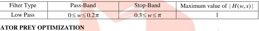
w are the weights. The design conditions for low pass digital FIR filter are presented in following table: Table 1: Conditions for the Design of Low Pass Digital FIR filter
Filter Type Pass-Band Stop-Band Maximum value of |H(w,x)|
Low Pass 0w0.2𝜋 0.3w𝜋 1
III. PREDATOR PREY OPTIMIZATION
Predator Prey Optimization technique is global search technique. Predator-prey model was first introduced by Silva et al. in 2002[1]. The motive behind the evolution of this model was to introduce diversity in the position of the swarms. It was concluded by Silva that PPO performs better than PSO because if initial parameters in PSO are chosen wrong it may trap in local minima. Furthermore, PPO is very valuable in clustering, as particles keep on moving, is extremely crucial, because the best position may not remain best after some time [3]. In this technique, particle swarm optimization (PSO) is added to the effect of the predator. PSO being population based technique utilizes the swarm intelligence like fish schooling, bird flocking. In this, the particle changes its position in accordance to the time which is based on its experience and experience of the neighbouring particles. The predator population is incorporated with the swarm particles in the model. The predator has different nature than the swarm particles; the predator gets attracted towards the best particle in the group, while repelling other particles. Prey particles always attempt to achieve best appropriate positions protecting from the attack of predator. Probability fear manages the impact of predator on any swarm particle. In PPO model, predator is used to search for global best in proper manner whereas preys search for a solution space running away from the predator’s attack, which helps to prevent immature convergence in local optima. In a condition when prey is attacked by the predator, an exponential term is combined with velocity vector [7].
Initializing position of population and velocity of population
The prey position and predator position is initialized randomly with Np preys along with an individual predator. 𝑥𝑖𝑘0 is prey position and 𝑥𝑝𝑖0 is predator position which are given as follows:
𝑥𝑖𝑘0 = 𝑥𝑖𝑚𝑖𝑛+ 𝑅𝑖𝑘1(𝑥𝑖𝑚𝑎𝑥− 𝑥𝑖𝑚𝑖𝑛)(𝑖 = 1,2, … , 𝑆; 𝑘 = 1,2, … , 𝑁𝑝) (10)
𝑥𝑝𝑖0 = 𝑥𝑖𝑚𝑖𝑛+ 𝑅2𝑖(𝑥𝑖𝑚𝑎𝑥− 𝑥𝑖𝑚𝑖𝑛)(𝑖 = 1,2, … , 𝑆) (11)
where 𝑥𝑖𝑚𝑖𝑛 is lower limit and 𝑥
𝑖𝑚𝑎𝑥 is upper limit for ith position of decision variables. 𝑅𝑖𝑘1 and 𝑅𝑖2 are uniform random numbers with values in interval(0, 1). 𝑆 denotes number of variables.𝑉𝑖𝑘0is the prey velocity and 𝑉𝑝𝑖0 is the predator velocity as defined below:
𝑉𝑖𝑘0 = 𝑉𝑖𝑚𝑖𝑛+ 𝑅𝑖𝑘1(𝑉𝑖𝑚𝑎𝑥− 𝑉𝑖𝑚𝑖𝑛)(𝑖 = 1,2, … , 𝑆; 𝑘 = 1,2, … , 𝑁𝑝) (12)
𝑉𝑝𝑖0 = 𝑉𝑝𝑖𝑚𝑖𝑛+ 𝑅2𝑖(𝑉𝑝𝑖𝑚𝑎𝑥− 𝑉𝑝𝑖𝑚𝑖𝑛)(𝑖 = 1,2, … , 𝑆) (13)
The value of maximum velocity as well as minimum velocity of prey can be set by using following equations where value of
𝛼 equals to 0.25.
𝑉𝑖𝑚𝑖𝑛 = −𝛼(𝑥𝑖𝑚𝑎𝑥− 𝑥𝑖𝑚𝑖𝑛)(𝑖 = 1,2, … , 𝑆) (14)
𝑉𝑖𝑚𝑎𝑥 = +𝛼(𝑥𝑖𝑚𝑎𝑥− 𝑥𝑖𝑚𝑖𝑛)(𝑖 = 1,2, … , 𝑆) (15)
IJEDR1603067
International Journal of Engineering Development and Research (www.ijedr.org)417
Evaluation of predator velocity and predator position
The predator velocity and predator position updates for (𝑡 + 1)𝑡ℎ movement are given as:
𝑉𝑃𝑖𝑡+1 = 𝐶4(𝐺𝑃𝑏𝑒𝑠𝑡𝑖𝑡− 𝑃𝑃𝑖𝑡) (𝑖 = 1,2, … , 𝑆) (16)
𝑥𝑃𝑖𝑡+1= 𝑥𝑃𝑖𝑡 + 𝑉𝑃𝑖𝑡+1(𝑖 = 1,2, … , 𝑆) (17)
Where 𝐺𝑃𝑏𝑒𝑠𝑡𝑖𝑡 is global best position of ith variable, 𝐶
4 is random number that lies between 0 and upper limit.
Evaluation of prey velocity and prey position
The velocity and position updates of prey for (𝑡 + 1)𝑡ℎ movement are given as:
𝑉𝑖𝑘𝑡+1 = {
𝑤𝑉𝑖𝑘𝑡 + 𝐶
1𝑅1(𝑥𝑏𝑒𝑠𝑡𝑖𝑘𝑡 − 𝑥𝑖𝑘𝑡) + 𝐶2𝑅2(𝐺𝑃𝑏𝑒𝑠𝑡𝑖𝑘𝑡 − 𝑥𝑖𝑘𝑡) ; 𝑃𝑓 ≤ 𝑃𝑓𝑚𝑎𝑥
𝑤𝑉𝑖𝑘𝑡 + 𝐶1𝑅1(𝑥𝑏𝑒𝑠𝑡𝑖𝑘𝑡 − 𝑥𝑖𝑘𝑡) + 𝐶2𝑅2(𝐺𝑃𝑏𝑒𝑠𝑡𝑖𝑘𝑡 − 𝑥𝑖𝑘𝑡) + 𝐶3𝑎(𝑒−𝑏𝑒𝑘); 𝑃𝑓 > 𝑃𝑓𝑚𝑎𝑥
(𝑖 = 1,2, … , 𝑆; 𝑘 = 1,2, … 𝑁𝑝) (18)
𝑥𝑖𝑘𝑡+1= 𝑥𝑖𝑘𝑡 + 𝑐𝑓𝑐𝑉𝑖𝑘𝑡+1 (𝑖 = 1,2, … , 𝑆; 𝑘 = 1,2, … 𝑁𝑝) (19)
where 𝐶1and 𝐶2 are acceleration constants; 𝑤 is inertia weight; Random numbers𝑅1 and 𝑅2are in range (0,1); 𝑥𝑏𝑒𝑠𝑡𝑖𝑘𝑡 is local finest position at kth population and ith variable; 𝐶
3 being a random number have value in interval (0, 1); constant ‘a’ is maximum amplitude of effect of predator on prey and ‘b’ is used for controlling the effect; 𝑒𝑘 is Euclidean distance lying between the position of prey and predator for kth population which is described as:
𝑒𝑘 = √∑𝑆𝑖=1(𝑥𝑖𝑘− 𝑥𝑝𝑖)2 (20)
𝑤 is inertia weight which is computed by:
𝑤 = [𝑤𝑚𝑎𝑥− (𝑤𝑚𝑎𝑥− 𝑤𝑚𝑖𝑛)(𝑡/𝑡
𝑚𝑎𝑥)] (21)
𝐶𝑓𝑐 is a constriction factor given by following equation:
𝐶𝑓𝑐= {|2 − ∅ − √∅
2− 4∅| 𝑖𝑓 ∅ ≥ 4
1 𝑖𝑓 ∅ < 4 (22)
The elements of prey positions and velocities may offend their limits. So, values are updated to set their violation as below:
𝑉𝑖𝑘𝑡 = {
𝑉𝑖𝑘𝑡 + 𝑅3𝑉𝑖𝑚𝑎𝑥 ; 𝑖𝑓 𝑉𝑖𝑘𝑡 < 𝑉𝑖𝑚𝑖𝑛
𝑉𝑖𝑘𝑡 − 𝑅3𝑉𝑖𝑚𝑎𝑥 ; 𝑖𝑓 𝑉𝑖𝑘𝑡 > 𝑉𝑖𝑚𝑎𝑥
𝑉𝑖𝑘𝑡 ; 𝑛𝑜 𝑣𝑖𝑜𝑙𝑎𝑡𝑖𝑜𝑛 𝑜𝑓 𝑙𝑖𝑚𝑖𝑡𝑠
(23)
𝑅3is any random number in the range 0 and 1. The process is repeated until the limits are satisfied.
Opposition Based Strategy
Normally, optimization techniques introduce some initial solutions and these solutions are improved to achieve best solutions. The process of searching is terminated, after satisfying some predefined criteria. Usually it is initiated with random guesses in the absence of preceding information about the solution. The computational time is distance between the initial guess and best solution. It can enhance the chance to start with best solution by concurrently analyzing the opposite solution. Due to this process, the superior one either the guess or the opposite guess can be selected as initial solution. According to probability theory, 50% of the time, the guess is far away from the solution as compared to its opposite guess. Thus, starting with closest to both guesses, it has ability to accelerate convergence. The similar approach can be applied to all solutions in the present population [2].
𝑥𝑘+𝑁𝑡 𝑝,𝑗= 𝑥
𝑖𝑚𝑖𝑛+ 𝑥𝑖𝑚𝑎𝑥− 𝑥𝑖𝑘𝑡 (𝑖 = 1,2, … , 𝑆; 𝑘 = 1,2, … , 𝑁𝑝) (24)
where, 𝑥𝑖𝑚𝑖𝑛is lower limit of filter coefficients and 𝑥𝑖𝑚𝑎𝑥 is upper limit of filter coefficients.
Algorithm for Predator Prey Optimization:
1. Specify the input data like size of swarm, maximum movements, maximum probability fear (Pfmax), highest and lowest limit of velocity of predator and prey.
2. Initialize the positions and velocities of prey and predator randomly. 3. Apply opposition based strategy.
4. Calculate the objective function. 5. Select Np preys for total 2Np preys.
6. Assign all the positions of the prey as their local finest position. 7. Calculate the global finest position from all local finest positions. 8. Update predator position and predator velocity.
9. Generate probability fear (pf) randomly between (0, 1). 10. If (pf > maximum pf)
Then
Predator affect is added while updating prey velocity along with prey position Else
Predator affect is not added while updating prey velocity along with prey position Endif.
11. Calculate the objective function of all population of prey. 12. Update local finest position of particles of prey.
IJEDR1603067
International Journal of Engineering Development and Research (www.ijedr.org)418
15. HaltIV. SIMULATION RESULTS
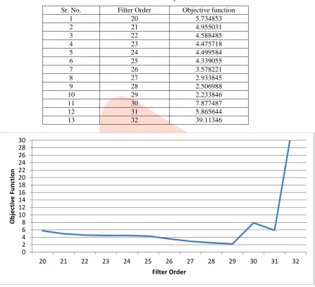
The digital low pass FIR filter has been designed with Predator Prey Optimization technique. In the designing of the filter, initially best filter order has been evaluated and then control parameters like population size and acceleration constants has been varied. In this technique, each program is made to run 100 times. The value of constant ‘a’ which represents maximum amplitude of effect of predator on prey is 0.0007× 𝑥𝑖𝑚𝑎𝑥 and constant ‘b’ for controlling the effect is 0.007/𝑥𝑖𝑚𝑎𝑥. Initially PPO has been implemented from 20 to 32 filter order. Different values of objective functions have been observed on different filter orders as shown below.
Table 2: Filter order and Objective function Sr. No. Filter Order Objective function
1 20 5.734853
2 21 4.955031
3 22 4.588485
4 23 4.475718
5 24 4.499584
6 25 4.339055
7 26 3.578221
8 27 2.933845
9 28 2.506988
10 29 2.233846
11 30 7.877487
12 31 5.865644
13 32 39.11346
Figure 1: Graph between Filter Order and Objective Function
As seen in the Fig. 1, objective function keeps on decreasing from filter order 20 to 29.Next to filter order 29, objective function rise steeply to very high value. Thus it is observed that filter order 29 has been selected as best order for designing low pass digital FIR filter having minimum objective function.
Now, two control parameters i.e. population size and acceleration constants have been varied on filter order 29. First of all, population size has been varied from 50 to 140. Best population has been selected using opposition based strategy. The values of objective function at different populations are depicted in the Table 3.
Table 3: Objective Function versus Population Size at filter order 29 Sr. No. Population Size Objective Function
1 50 2.234328
2 60 2.234167
3 70 2.233865
4 80 2.233862
5 90 2.233876
0 2 4 6 8 10 12 14 16 18 20 22 24 26 28 30
20 21 22 23 24 25 26 27 28 29 30 31 32
Ob
jec
tiv
e
Fu
n
ction
IJEDR1603067
International Journal of Engineering Development and Research (www.ijedr.org)419
6 100 2.233846
7 110 2.263915
8 120 2.304246
9 130 2.310894
10 140 2.310948
The variation in objective function slightly decreases for population from 50 to 100, and after that objective function raises abruptly. So, it observed that population size of 100 gives minimum objective value.
Figure 2: Graph of Objective Function versus Population Size at filter order 29
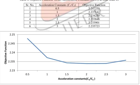
Another control parameter that is acceleration constants C1/C2 has been varied on population size 100. The value of both C1 and C2 is kept equal and objective function has been being calculated. The value of C1/C2 has been taken as depicted in the Table 4.
Table 4: Objective Function versus Acceleration Constants (C1/C2) at filter order 29 Sr. No. Acceleration Constants (C1/C2) Objective Function
1 0.5 2.247773
2 1 2.237142
3 1.5 2.234250
4 2 2.233846
5 2.5 2.233901
6 3 2.235723
Figure 3: Graph of Objective function versus Acceleration Constants (C1/C2) at filter order 29
It has been examined from Fig. 3 that the acceleration constants C1/C2 have been varied. The objective function gradually decreases for the value of C1/C2 from 0.5 to 1.5, and then it slightly decreases from 1.5 to 2. Further acceleration constant
2.23 2.2352.24 2.2452.25 2.2552.26 2.2652.27 2.2752.28 2.2852.29 2.2952.3 2.3052.31 2.315
50 60 70 80 90 100 110 120 130 140
Ob
jec
tiv
e
Fu
n
ction
Population
2.23 2.235 2.24 2.245 2.25
0.5 1 1.5 2 2.5 3
Ob
jec
tiv
e
Fu
n
ction
IJEDR1603067
International Journal of Engineering Development and Research (www.ijedr.org)420
increases. Thus, it has been observed that minimum value of objective function is achieved when value of C1/C2 is 2. It is very clear in the given graph.The algorithm has been run for 200 iterations which is defined as the stopping criterion. The objective function for 200 iterations has been given in Fig. 4.
Figure 4: Graph of Objective function versus Iterations
It has been examined that the value of objective function first declines up to 10th iteration and then it remains constant for the rest of iterations.
From the results it is clear that PPO is better than PSO because in design of low pass filter using PSO, it was observed that best results were obtained at filter order 28 [10]. But with use of PPO better results has been obtained at filter order 28 and further much better results has been obtained at filter order 29with reduced value of magnitude errors e1, e2 and pass band ripple error. It improves conflicting nature of pass-band ripple and stop-band ripple.
Table 5: Comparison of Values of Magnitude errors and Pass band ripple error of PSO and PPO Technique Used Filter
Order
Sr. No. Objective Function Magnitude Error (e1)
Magnitude Error (e2)
Pass Band Ripple Error PSO
[10]
28 1 2.690961 1.410883 0.173005 0.059919
PPO 28 2 2.506988 1.332099 0.172858 0.048945
PPO 29 3 2.233846 1.153304 0.148559 0.048512
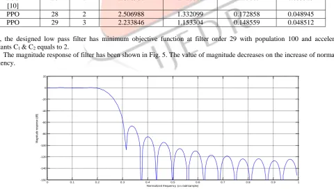
Thus, the designed low pass filter has minimum objective function at filter order 29 with population 100 and acceleration constants C1 & C2 equals to 2.
The magnitude response of filter has been shown in Fig. 5. The value of magnitude decreases on the increase of normalized frequency.
Figure 5: Magnitude Response versus Normalized Frequency at filter order 29
The phase response has been varied corresponding to the normalized frequency for filter order 29 to design low pass digital FIR filter. The graph has been shown as follows in Fig. 6.
2 2.2 2.4 2.6 2.8 3 3.2
0 20 40 60 80 100 120 140 160 180 200
Ob
jec
tiv
e
Fu
n
ction
Iterations
0 0.1 0.2 0.3 0.4 0.5 0.6 0.7 0.8 0.9 1 -160
-140 -120 -100 -80 -60 -40 -20 0 20
M
ag
ni
tu
de
r
es
po
ns
e
(d
B
)
IJEDR1603067
International Journal of Engineering Development and Research (www.ijedr.org)421
Figure 6: Phase Response with respect to Normalized Frequency at filter order 29The graph of magnitude versus normalized frequency has been given in Fig. 7. The low pass digital filter first passes the low frequencies and attenuates high frequencies as shown.
Figure 7: Magnitude Response with respect to Normalized Frequency at filter order 29
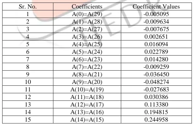
The absolute number of coefficients used in the designing is 30. Only half coefficients have been computed because filter has the property of symmetry. The coefficients at filter order 29 are given in Table 6 below:
Table 6: Optimized Coefficients of FIR Filter at filter order 29
Sr. No. Coefficients Coefficient Values
1 A(0)=A(29) -0.005095
2 A(1)=A(28) -0.009634
3 A(2)=A(27) -0.007675
4 A(3)=A(26) 0.002651
5 A(4)=A(25) 0.016094
6 A(5)=A(24) 0.022789
7 A(6)=A(23) 0.014280
8 A(7)=A(22) -0.009259
9 A(8)=A(21) -0.036450
10 A(9)=A(20) -0.048274
11 A(10)=A(19) -0.027683
12 A(11)=A(18) 0.030386
13 A(12)=A(17) 0.113380
14 A(13)=A(16) 0.194815
15 A(14)=A(15) 0.244958
Table 7: Analytical calculation of Objective Function as well as Standard Deviation Sr. No. Maximum value of
Objective Function
Minimum value of Objective Function
Average value of Objective Function
Standard Deviation
1 2.2912 2.233846 2.238068 0.040555
It is clear from the Table 7 that standard deviation is less than 1, which reveals that the filter is robust in nature.
0 0.1 0.2 0.3 0.4 0.5 0.6 0.7 0.8 0.9 1 -15
-10 -5 0
P
h
a
s
e
r
e
s
p
o
n
s
e
(
d
e
g
re
e
s
)
Normalized frequency (x rad/sample)
0 0.1 0.2 0.3 0.4 0.5 0.6 0.7 0.8 0.9 1
0 0.1 0.2 0.3 0.4 0.5 0.6 0.7 0.8 0.9 1
M
a
g
n
it
u
d
e
r
e
s
p
o
n
s
e
IJEDR1603067
International Journal of Engineering Development and Research (www.ijedr.org)422
V. CONCLUSIONThe low pass digital FIR filter has been designed using predator prey optimization technique. In this paper, PPO has been implemented from 20 to 32 filter order. It has been examined that the best results are obtained at filter order 29. Then two control parameters i.e. population size and acceleration constants C1 and C2 have been varied in order to obtain better results. On varying these variables, it has been concluded that best results are obtained with population size 100 and value of acceleration constants C1 & C2 equals to 2.0. The variation of an objective function corresponding to iterations has been also plotted. Further simulation has been carried out in MATLAB. Plot of magnitude response and phase response has been studied. The standard deviation of objective function is less than one which proves robustness nature of digital low pass filter.
REFERENCES
[1] Arlindo Silva, Ana Neves and Ernesto Costa, (2002), “An Empirical Comparison of Particle Swarm and Predator Prey Optimisation”, Proc Irish International Conference on Artificial Intelligence and Cognitive Science, vol. 24, no. 64, pp. 103-110.
[2] Shahryar Rahnamayan, Hamid R. Tizhoosh and Magdy M. A. Salama, (2008), “Opposition-Based Differential Evolution”, IEEE Transactions on Evolutionary Computation, vol. 12, no. 1, pp. 64-79.
[3] R. K. Johnson and F. Sahin, (2009), “Particle swarm optimization methods for data clustering”, Fifth International Conference on Soft Computing, Computing with Words and Perceptions in System Analysis, Decision and Control, Famagusta, pp. 1-6.
[4] Ashok Ambardar, (2011), “Digital Signal Processing: A Modern Introduction”, CENGAGE Learning, Eighth edition. [5] Sonika Aggarwal, Aashish Gagneja and Aman Panghal, (2012), “Design of FIR filter using GA and its comparison with
Hamming window and Parks Mclellan Optimization techniques”, International Journal of Advanced Research in Computer Science and Software Engineering, vol. 2, no.7, pp. 132-137.
[6] Sonika Gupta and Aman Panghal, (2012), “Performance Analysis of FIR Filter Design by Using Rectangular, Hanning and Hamming Window Methods”, International Journal of Advanced Research in Computer Science and Software Engineering, vol. 2, no. 6, pp. 273-277.
[7] Balraj Singh, J. S. Dhillon and Y. S. Brar, (2013), “Predator Prey Optimization method for the Design of IIR Method”, WSEAS Transactions on Signal Processing, vol. 9, no. 2, pp. 51-63.
[8] John Proakis and Dimitris Manolakis, (2013), “Digital Signal Processing: Principles, Algorithms and Applications”, Person Prentice Hall, Fourth Edition.
[9] Sukhdeep Kaur Sohi and Balraj Singh Sidhu, (2015), “Design of Low Pass Digital FIR Filter using Different Mutation Strategies of Differential Evolution”, International Journal of Advanced Technology in Engineering and Science, vol. 3, no. 6, pp. 148-158.
[10] Gagandeep Kaur, Darshan Singh Sidhu and Amandeep Kaur, (2015), “Design and Analysis of Digital Low Pass FIR Filter using Particle Swarm Optimization”, International Journal for Electro Computational World Knowledge Interface, vol. 4, no.1, pp. 17-23.