Tweets About Tornado Warnings: A Spatiotemporal And Content Analysis

(1)

University of South Carolina

Scholar Commons

Theses and Dissertations

2018

Phylogeny, Ancestral Genome, And Disease

Diagnoses Models Constructions Using Biological

Data

Bing Feng

University of South Carolina - Columbia

Follow this and additional works at:https://scholarcommons.sc.edu/etd Part of theComputer Sciences Commons

This Open Access Dissertation is brought to you by Scholar Commons. It has been accepted for inclusion in Theses and Dissertations by an authorized administrator of Scholar Commons. For more information, please [email protected].

Recommended Citation

(2)

PHYLOGENY,

ANCESTRAL

GENOME,

AND

DISEASE

DIAGNOSES

MODELS

CONSTRUCTIONS

USING

BIOLOGICAL

DATA

by

Bing Feng

Bachelor of Engineering

Shandong University of Science and Technology, 2009

Master of Science

Capital Normal University, 2012

Submitted in Partial Fulfillment of the Requirements

For the Degree of Doctor of Philosophy in

Computer Science

College of Engineering and Computing

University of South Carolina

2018

Accepted by:

Jijun Tang, Major Professor

Homayoun Valafar, Committee Member

John Rose, Committee Member

Chin-Tser Huang, Committee Member

Yan Guo, Committee Member

(3)

(4)

ACKNOWLEDGEMENTS

I would like to gratefully and sincerely thank my advisor, Dr. Jijun Tang, for his

guidance, encouragements, and patients during my graduate studies. He gave me the best

guidance and supports to my study and research. He is not only a teacher, advisor to my

study and research, but also the best friend.

I would like to thank the professors of the Department of Computer Science and

Engineering for their inputs, valuable discussions. I would like to express special thanks to

my doctoral committee members. They gave me enormous advice, guidance, and help to

my study and research. It is an honor to have them in my committee.

Finally, I would like to express my gratitude and thanks to my family and friends.

I thank for their love, supports, and great confidences in me all through these years. I would

also like to thank all of the members of our research group, giving me important

suggestions and helps. It is my pleasure to work in our research group and cooperate with

(5)

ABSTRACT

Studies of bioinformatics develop methods and software tools to analyze the

biological data and provide insight of the mechanisms of biological process. Machine

learning techniques have been widely used by researchers for disease prediction, disease

diagnosis, and bio-marker identification. Using machine-learning algorithms to diagnose

diseases has a couple of advantages. Besides solely relying on the doctors’ experiences and

stereotyped formulas, researchers could use learning algorithms to analyze sophisticated,

high-dimensional and multimodal biomedical data, and construct prediction/classification

models to make decisions even when some information was incomplete, unknown, or

contradictory. In this study, first of all, we built an automated computational pipeline to

reconstruct phylogenies and ancestral genomes for two high-resolution real yeast whole

genome datasets. Furthermore, we compared the results with recent studies and

publications to show that we reconstruct very accurate and robust phylogenies, as well as

ancestors. We also identified and analyzed conserved syntenic blocks among reconstructed

ancestral genomes and present yeast species.

Next, we analyzed the metabolic level dataset obtained from positive mass

spectrometry of human blood samples. We applied machine learning algorithms and

feature selection algorithms to construct diagnosis models of Chronic kidney diseases

(6)

among the metabolite features and the developments of CKD stages. The selected

metabolite features provided insights into CKD early stage diagnosis, pathophysiological

mechanisms, CKD treatments, and medicine development.

Finally, we used deep learning techniques to build accurate Down Syndrome (DS)

prediction/screening models based on the analysis of newly introduced Illumina human

genome genotyping array. We proposed a bi-stream convolutional neural network (CNN)

architecture with ten layers and two merged CNN models, which took two input

chromosome SNP maps in combination. We evaluated and compared the performances of

our CNN DS predictions models with conventional machine learning algorithms. We

visualized the feature maps and trained filter weights from intermediate layers of our

trained CNN model. We further discussed the advantages of our method and the underlying

(7)

LIST OF FIGURES

Figure 2. 1 Yeasts phylogeny built from all types of evolutionary events from 11 yeast species. ... 19

Figure 2. 2 Yeasts phylogeny built from all types of evolutionary events from 20 yeast species. ... 21

Figure 2. 3 Genome content, gene adjacency and evolutionary events comparisons among PMAG09, MANUAL09, and MANUAL12 ancestors. ... 25

Figure 2. 4 Genome content, gene adjacency, and evolutionary events comparisons between PMAG12 and MANUAL12 ancestors. ... 27

Figure 2. 5 Results analyses and comparisons of different approaches on simulated genome datasets. ... 30

Figure 2. 6 Chromosome dot plots between our ancestors and the "benchmark" ancestor MANUAL12. ... 32

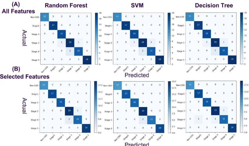
Figure 3. 1 Confusion matrices of the CKD stage classification/prediction models built from the same training and testing data set. ... 44

Figure 3. 2 Analyses of selected metabolites subset based on unsupervised learning algorithms. ... 49

Figure 3. 3 Correlation analyses among metabolites features and CKD stages. ... 51

Figure 4. 1 Chromosome SNP maps to represent the intensities of all SNP site

on HSA21. ... 57

Figure 4. 2 Detailed model configuration of the CNN architecture. ... 59

Figure 4. 3 CNN architecture built for DS prediction/screening model construction using chromosome SNP maps. ... 61

(10)

LIST OF TABLES

Table 2. 1 Binary encoding genome data. ... 14

Table 2. 2 Syntenic genes and blocks among ancestral genomes. ... 32

Table 2. 3 Syntenic genes and blocks between ancestral genomes and present yeast genomes ... 34

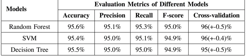
Table 3. 1 Performances of CKD stage diagnosis/classification models built from all metabolite features. ... 43

Table 3. 2 CKD stage diagnosis/classification models built from the selected metabolite features. ... 46

Table 4. 1 Evaluation metrics of bi-stream CNN and conventional machine learning models. ... 62

(11)

CHAPTER 1 INTRODUCTION

1.1 RELATED STUDIES ON PHYLOGENY AND ANCESTRAL GENOME

RECONSTRUCTION

Phylogenetic studies used to be the domain of morphological area and were based

on outward appearances and internal structures (Snodgrass, 1938). Later on, molecular

characters and DNA sequencing technologies had augmented these studies in building

robust phylogenies (Frickey & Lupas, 2004; Höhl & Ragan, 2007), however, different

methods often yielded conflicting phylogeny results (Hedtke, Townsend, & Hillis, 2006;

Marcet-Houben & Gabaldón, 2015; Rokas, King, Finnerty, & Carroll, 2003; Salichos &

Rokas, 2013; Vakirlis et al., 2016). Local and biased sequences may not be enough to

conflicting phylogenetic signals. Currently, the widely accepted phylogenetic approach to

alleviate these conflicting issues is to analyze shared gene datasets, and

concatenate/coalesce their results from multiple sequence alignments to obtain a final

phylogeny with the maximum support (Marcet-Houben & Gabaldón, 2015; Salichos &

Rokas, 2013; Vakirlis et al., 2016). Recently, Salichos et al. analyzed a yeast gene dataset

with 1,070 orthologs from 23 species and discovered 1,070 phylogenies. They

(12)

& Rokas, 2013). Marcet-Houben and Vakirlis also used similar approaches to build yeast

phylogenies for 19 and 34 species (Marcet-Houben & Gabaldón, 2015; Vakirlis et al.,

2016). Nevertheless, contradictories still exist among these studies. These conflicting

phylogenies could be caused by method inconsistency, compositional bias, alignment

ambiguity, model misspecification, and long branches attraction (Hedtke et al., 2006;

Salichos & Rokas, 2013).

Genome-level evolutionary events and their biological significances have been

studied for 80 years (Sturtevant & Dobzhansky, 1936). Computational methods were

developed in 1990s (Blanchette, Bourque, & Sankoff, 1997; Sankoff & Blanchette,1997).

Since then, computational methods were widely explored in phylogeny reconstructions and

evolutionary mechanisms in the past three decades (Avdeyev, Jiang, Aganezov, Hu, &

Alekseyev, 2016; Ma, 2010; Perrin, Varré, Blanquart, & Ouangraoua, 2015; Sankoff, 2009;

Sankoff & Zheng, 2013; Xu & Moret, 2011). The availability of fully sequenced/annotated

genomes and advanced computational algorithms have brought evolutionary studies going

beyond the mere sequence level (Boore, 2006; Fertin, 2009). Gene orders can be used as

genome markers in genome level evolutionary studies (Delsuc, Brinkmann, & Philippe,

2005). They represent the genome content, gene permutations, and gene directions, which

can reflect genome content and structural variations during evolution. Gene order-based

phylogeny reconstruction approaches obtain phylogenetic signals from genome level

evolutionary events and can bypass the troublesome multiple sequence alignment step in

traditional methods (Boore, 2006; Fertin, 2009; Lin, Hu, Tang, & Moret, 2013). However,

gene order level phylogenetic studies are more computationally costly when compared with

traditional sequence level studies. Because researchers usually treat all gene order

(13)

permutation states (Avdeyev et al., 2016; Fertin, 2009; Hu, Zhou, Zhou, & Tang, 2014;

Vakirlis et al., 2016; L. Zhou, Hoskins, Zhao, & Tang, 2015).

Researchers have been working on the computational approaches for phylogeny

and ancestral reconstructions on whole genome level data (Avdeyev et al., 2016; Gagnon,

Blanchette, & El-Mabrouk, 2012; Gao, Zhang, Feng, & Tang, 2015; Lin et al., 2013;

Sankoff & Zheng, 2013; Xu & Moret, 2011; J. Zhou et al., 2016; L. Zhou et al., 2015; L.

Zhou, Lin, Feng, Zhao, & Tang, 2016). Most present approaches can only handle simplified

real genome datasets or simulated datasets with identical genome content and unique

genome markers (Alekseyev & Pevzner, 2009; Feijão & Meidanis, 2009; Hu, Zhou, &

Tang, 2013; Ma, 2010; Perrin et al., 2015; Xu & Moret, 2011; Zheng & Sankoff, 2011).

So that they cannot be applied to the original real genome data without modifications. They

are also restricted by handling complex evolutionary events, such as deletion, insertion,

and duplication (Avdeyev et al., 2016; Feijão & Meidanis, 2009; Feng, Zhou, & Tang,

2017; Ma, 2010; Perrin et al., 2015; Xu & Moret, 2011; L. Zhou et al., 2015). Some recent

studies used the modified real genome datasets to build phylogenies, by removing

non-shared genes (Luo et al., 2012) or using mitochondrial data (Figueroa & Baco, 2015;

Weigert et al., 2016). For current computational ancestral reconstruction methods, only

ANGES (Jones, Rajaraman, Tannier, & Chauve, 2012), Gapped Adjacency (Gagnon et al.,

2012), and MGRA2 (Avdeyev et al., 2016) are reported being able to hand non-identical

genome content and all types of evolutionary events. However, they still suffer from issues

of low-resolution, accuracy, and robustness. Recently, gene duplication events have also

been considered in real genome ancestral reconstructions, but only for X-chromosome of

(14)

Yeasts have been used as models for higher level complex organisms, including

mammals and humans (Bhargava, 2010). Whole-genome sequencing studies have shown

that yeasts have similar genome sizes, gene contents, and collinearity of genes along the

chromosomes of species (Wolfe, 2015). Gordon reconstructed the yeast ancestral genome

that extinct 100 million years ago with a manual approach, using the gene order data of 11

species in Yeast Genome Order Browser (YGOB) (http://ygob.ucd.ie) (Byrne & Wolfe,

2005; Gordon, Byrne, & Wolfe, 2009). In the latest version of YGOB, Byrne and Wolfe

added nine additional yeast species and reconstructed a ’benchmark’ version of yeast

ancestral genome from 20 species using the same method (Byrne & Wolfe, 2005; Gordon

et al., 2011). Jean proposed a computational method to reconstruct an ancestral genome for

five non-WGD (Whole-genome duplication) species in YGOB (Jean, Sherman, &

Nikolski, 2009). Chauve later developed a computational method to reconstruct an

ancestral genome using the same dataset as Jean but with two genome marker sets (Chauve,

Gavranovic, Ouangraoua, & Tannier, 2010). The “low-resolution marker set” contains the

same 135 genome makers that were used by Jean. (Jean et al., 2009) The “high-resolution

marker set” contains 710 genome markers (Chauve et al., 2010). However, their studies are

still based on low-resolution datasets with only five species. Even the "high-resolution set"

with 710 markers is still too low to reconstruct reliable ancestral architectures for current

whole genome level studies. Vakirlis reconstructed yeast ancestral genomes from 10

non-WGD species of the Lachancea genus. They annotated 3,598 orthologs among these 10

species and considered each gene as a genome marker to reach the highest resolution.

However, their studies are only limited in one non-WGD genus. (Vakirlis et al., 2016)

Our group previously developed two computational phylogeny and ancestral

(15)

et al., 2013) and PMAG (Probabilistic Method of Ancestral Genomics) (Hu et al., 2013).

These approaches could only handle simulated data with identical genome content, unique

genome markers, and limited types of evolutionary events. In this study, we redesigned the

evolutionary models and innovated the algorithms for these two approaches. Our improved

approaches now can handle real genome data, which have non-identical genome contents,

non-unique genome markers, and all types of evolutionary events, including genome

rearrangements, insertion, deletion, duplication, and whole genome duplication (WGD).

Furthermore, we built an automated pipeline to reconstruct phylogenies and ancestral

genomes for two high-resolution whole-genome datasets of the Saccharomycetaceae

family. Finally, we identified and analyzed conserved syntenic blocks among reconstructed

ancestors and present yeast species.

1.2 RELATED STUDIES ON CKD SCREENING AND DIAGNOSIS

Chronic Kidney Diseases (CKDs) are progressive losses and abnormalities of

kidney functions and structures (Levey et al., 2005). Now they become major challenges

to public health and affect approximately 10% of the population worldwide (Subasi,

Alickovic, & Kevric, 2017). CKDs often result in Acute Kidney Injury (AKI), which

appears abruptly and has rapid deterioration of kidney function (Bellomo, Kellum, &

Ronco, 2012; Chawla, Eggers, Star, & Kimmel, 2014). The end-stage (stage 5) and AKI

would cause renal failure and require special treatments such as dialysis and renal

transplant (Bagshaw, Berthiaume, Delaney, & Bellomo, 2008). CKDs are also associated

with other severe complications, including cardiovascular disease, hypertension, diabetes

(Levey et al., 2003), cognitive decline, anemia, mineral and bone disorders, and fractures

(Jha et al., 2013). CKD screening and stage detection are critical to the prognosis and

(16)

treated in the early stage (Levey et al., 2003; Morton, Tong, Howard, Snelling, & Webster,

2010). Prompt treatments and management for specific CKD stages can significantly

prevent and delay the promotions and progressions of CKDs. (Jha et al., 2013; Levey et

al., 2003; Morton et al., 2010). Meanwhile, CKDs in different stages require different

management, treatments, and medicines (Coresh et al., 2007; Lameire & Van Biesen, 2010;

Levey & Coresh, 2012). Proper management strategies can significantly reduce the

incidence of end-stage CKDs. (Jha et al., 2013). However, the early stage of CKD (stage

1) is hard to be recognized (Levey et al., 2013) because initially, no symptoms might be

found. Treatments and management for CKD will not be made until symptoms become

severe or accidental findings from tests for other diseases (Webster et al., 2017).

Recent international guidelines classify CKDs into five stages based on the levels

of glomerular filtration rate (GFR) (Levey et al., 2005, 2013). GFR is computed by

estimating equations and other associated exogenous bio-factors (Webster et al., 2017). In

fact, there are many issues in current GFR estimation approaches. The estimating equations

may lead to inaccuracy due to the patient's’ personal situations including age, race, gender,

and serum creatinine level (Levey et al., 2002, 2005; Levin et al., 2013). Moreover, various

GFR estimating approaches and equations will result in disagreements and errors for the

same patients (Bevc et al., 2017). Recent Bland-Altman analysis showed that the

CKD-EPI creatinine-cystatin C, BIS2, CKD-CKD-EPI cystatin C and Simple cystatin C GFR equations

were all lacking accuracies in estimating GFR for elderly people (Bevc et al., 2017).

Researchers also discovered that using the Schwartz formula to estimate GFR for children

would result in overestimations (Levey et al., 2009). Muna et al. found that the BIS

equation was not a proper approach to predict the risks of death for older women when

(17)

contradictory issues in present GFR estimating approaches might result in misjudgement

of CKD stages, which may cause further underdiagnoses and undertreatments (Levey et

al., 2003).

Using machine learning algorithms to diagnose diseases has a few advantages.

Besides solely relying on the doctors’ experiences and stereotyped formulas, researchers

could use learning algorithms to analyze sophisticated, high-dimensional and multimodal

biomedical data, and construct prediction/classification models to make decisions even

when some information was incomplete, unknown, or contradictory. Current

machine-learning based CKD diagnostic studies have shown high accuracies and reliabilities in

CKDs detections and diagnoses (Polat, Mehr, & Cetin, 2017). Neves et al. used Artificial

Neural Networks to build a classification model to classify 558 CKD and non-CKD

patients based on 24 features, which achieved 92.3 % accuracy in testing (Neves et al.,

2015). Celik et al. used Decision Tree and Support Vector Machine (SVM) algorithms to

classify a CKD dataset with 400 patients and 24 features, which both achieved accuracies

over 96% in classifying the CKD and non-CKD patients (Celik, Atalay, & Kondiloglu,

2016). Polat et al. used the SVM algorithm to classify the same CKD dataset used by Celik,

which reached an accuracy of 98.5% (Polat et al., 2017). Chen et al applied three different

learning algorithms to construct classification models for the datasets with CKD and

non-CKD patients, which all achieved accuracies over 93% (Chen, Zhang, & Zhang, 2016).

However, most present CKD diagnosis machine learning studies performed only on small

datasets with limited numbers of physiological features. They only focused on the simple

yes/no problems but could not classify the different CKD stages (Celik et al., 2016; Neves

(18)

1.3 RELATED STUDIES ON DOWN SYNDROME SCREENING

Down syndrome (DS) is a genetic disorder caused by genome dosage imbalances

and micro-duplications of human chromosome 21 (HSA21) (Antonarakis, 2016). It is

usually associated with intellectual disability, congenital heart defects, childhood

leukaemia, Alzheimer’s disease, early ageing, physical abnormalities, and other

abnormalities (Antonarakis, 2016; Patterson, 2009; Wiseman, Alford, Tybulewicz, &

Fisher, 2009) Even though DS happens at a high rate worldwide (1 per 1,000 live births)

(Weijerman & De Winter, 2010), and has been well studied, researchers haven’t found any

effective cure method. No environmental factors or parents’ behavioral factor has been

discovered to cause the Human DS disease either (Parker et al., 2010). Currently, DS

therapies in human studies mainly concentrate on early intervention, educational therapy

(Guralnick, 2010; Wuang, Chiang, Su, & Wang, 2011), physical therapy (Chavez, 2016;

Wentz, 2017), as well as emotional and behavioral therapies (Greenspan, Wieder, &

Simons, 1998; Wuang et al., 2011). These therapies only have limited effects and can

barely cure DS fundamentally. Therefore, Screening and early detection become the most

efficient way of DS prevention.

DS screening has been studied since 1960s. A few DS biomarkers have been

discovered, such as alpha-fetoprotein levels, human chorion gonadotropin, and

unconjugated estriol (Brock & Sutcliffe, 1972; Wald et al., 1988). Currently, the most

widely used approaches for DS screening include ultrasound measurement of fetal nuchal

translucency (Spencer, Souter, Tul, Snijders, & Nicolaides, 1999), blood test (Ehrich et al.,

2011), sequencing test (Palomaki et al., 2011), and combined genetic test (Driscoll &

(19)

high-risk invasive diagnostic procedures, such as amniocentesis and chorionic villus

sampling, which both have a 1/200 chance to result in the fetal loss (Palomaki et al., 2011).

Human chromosome 21 (Hsa21) encodes more than 500 genes (Higuera, Gardiner, & Cios,

2015; Sturgeon & Gardiner, 2011), including protein modifiers, transcription factors, RNA

splicing factors/modifiers, cell surface receptors and adhesion molecules, and components

of many biochemical pathways (Dierssen & de la Torre, 2012; Higuera et al., 2015).

However, only 165 genes are annotated as protein-coding genes or microRNAs. More than

350 genes have unassigned functions (K. Gardiner et al., 2010). Recent GWAS studies

have discovered that the SNPs (Single-nucleotide polymorphisms) variation, copy number

variations, and unidentified genetic variation are highly correlated with human DS (Jain et

al., 2016; Petry et al., 2017; Ramachandran et al., 2015; Sailani et al., 2013). Illumina has

introduced a new exome genotyping array technique that targets the exome plus rare

single-nucleotide polymorphisms (SNPs). The Vanderbilt Epidemiology Center and Center for

Quantitative Sciences developed a chip–processing protocols and collected the clinical

genotyping data for various diseases (Sailani et al., 2013).

Mice models can be used to dissect the Hsa21 gene interactions and study the DS

phenotype. Experimental pathway perturbations studies on the mouse model with

segmental trisomy for Hsa21 provide unprecedented opportunity to decipher human DS

pathway studies (K. Gardiner et al., 2010). Ts65Dn mice model has three copies of over

half of the Hsa21 orthologs genes on chromosome 16 (Reinholdt et al., 2011), and it a

widely used DS model of human DS (Kuehn, 2016). Some achievements have been

accomplished in the DS therapies in mouse models. Laura et al found that prenatal

treatments with NAPVSIPQ and SALLRSIPA could prevent developmental delay and glial

(20)

in synaptic and cognitive dysfunction. Its reduction could restore the Kir3.2 hippocampal

level to normal. (Kleschevnikov et al., 2017)

Machine learning techniques have been used in diseases diagnosis, diseases related

genetic disorder, and bio-marker predictions (Gray et al., 2013; Park & Kellis, 2015; Roth

et al., 2016). Commonly used supervised learning methods include Conventional artificial

neural network, Deep learning neural networks, Support vector machine (SVM) (Roth et

al., 2016), random forest (Gray et al., 2013), decision tree (Anbarasi, Anupriya, & Iyengar,

2010), and Bayesian classifiers (Schwarz, Rödelsperger, Schuelke, & Seelow, 2010).

Recently, deep convolutional neural networks (CNN) and recurrent neural networks

(RNN) have achieved impressive results in a variety of disease screening, diagnosis, and

predictions problems (Esteva et al., 2017; Faust et al., 2016; Roth et al., 2016; Sun, Tseng,

Zhang, & Qian, 2017). Based on our knowledge, only a few conventional machine learning

techniques have been applied to human DS studies (Higuera et al., 2015). Most of them

performed on DS mice model Ts65Dn (Higuera et al., 2015; Nguyen, Costa, Cios, &

Gardiner, 2011; Sailani et al., 2013). Clara et al. analyzed the expression levels of 77

proteins and designed an unsupervised self-organizing map to identify biological

differences of DS mice model Ts65Dn (Higuera et al., 2015). Cao et al. used a naïve Bayes

classifier to predict the level of locomotor activity under the treatments of the

N-methyl-D-aspartate receptor in mice models Ts65Dn and Ts1Cje (Nguyen et al., 2011). Zhao et al.

proposed a hierarchical constrained local model with independent component analysis to

(21)

CHAPTER 2 PHYLOGENY AND ANCESTOR RECONSTRUCTION USING YEASTS

GENOME DATA

2.1 MOTIVATIONS

Originally, studies of yeast phylogenies were based on morphological phenotypes

and characters, such as sexual states, germinations, and fermentations (Kurtzman, Fell, &

Boekhout, 2011). Currently, widely accepted yeasts phylogenetic approaches are based on

multiple sequence alignment. However, there are still limitations and common conflicting

results with each other (Hedtke et al., 2006; Marcet-Houben & Gabaldón, 2015; Salichos

& Rokas, 2013; Vakirlis et al., 2016). Current whole genome level phylogenetic studies on

real data are limited in simplified identical content genomes (Luo et al., 2012) and

mitochondrial datasets (Figueroa & Baco, 2015; Weigert et al., 2016). In this study, we

want to reconstruct the phylogenies for two high-resolution yeasts genome datasets by

using phylogenetic signals from genome level evolutionary events. We will compare our

results with the NCBI taxonomy and recent publications. We will provide a new and

alternative method to resolve the same phylogenetic problems by using different types of

(22)

Reconstructing ancestral genomes offers opportunities to study the evolutionary

mechanisms and trajectories of present species. Studies focused on developing

computational ancestor reconstruction approaches are facing many difficulties. Present

computational approaches are suffering from issues of simplistic evolutionary models,

complex datasets, and complex evolutionary events (Feng et al., 2017; Gao et al., 2015;

Ma, 2010; Perrin et al., 2015; Sankoff, 2009; Xu & Moret, 2011; L. Zhou et al., 2016). We

will build an automated pipeline to reconstruct phylogenies and ancestral genomes from

the whole genome data. First, we will build the phylogenies, and use them as guide trees

to reconstruct ancestral genomes from the same input data.

The whole genome level evolutionary studies will improve our understanding of

evolutionary procedures, gene origins, and gene co-evolutions (Boore, 2006; Sankoff,

2009). Studies of syntenic blocks in gene order level have several applications in analyzing

the genome’s structural and functional evolutions (Sankoff, 2009). We will identify the

syntenic blocks by analyzing the correlations between evolutionary events and these

functional variations. We can use syntenic blocks as genome markers to detect critical

evolutionary events, such as functional gene gain and loss. We can also study the genotypes

and phenotypes of ancestral genomes that have gone extinct. Annotated gene orders within

shared syntenic blocks can be used to locate the orthologous genes across different species.

We can use them to trace the gene origins, evolutionary paths, and functional variations in

(23)

2.2 METHODOLOGY

2.2.1 Yeast Genome Dataset

In this study, we reconstructed phylogenies and ancestral genomes for two yeast

whole genome datasets. Both datasets are available in the Yeast Gene Order Browser

(YGOB) (http://ygob.ucd.ie) (Byrne & Wolfe, 2005). The first dataset contains the genome

data of 11 yeast species (Version 3, April 2009), including five post-WGD species under

four genera (S.cerevisiae, S.uvarum, C.glabrata, N.castelliie, V.polyspora), and six

non-WGD species under four genera (Z.rouxii, K.lactis, E.gossypii, L.kluyveri,

L.thermotolerans and L.waltii). This is the same dataset that were used in Gordon’s study

for reconstructing yeast ancestor (Byrne & Wolfe, 2005; Gordon et al., 2009). The second

yeast dataset is also available in YGOB (Version 7, August 2012), and contains nine

additional species compared to the first dataset (Byrne & Wolfe, 2005; Gordon et al.,

2011). Twelve species are post-WGD species under six genera (S.uvarum, S.kudriavzevii,

S.mikatae, S. cerevisiae, V.polyspora, T.phaffii, T.blattae, N.dairenensis, N.castellii,

K.naganishii, K.africana, C.glabrata). Eight species are non-WGD species under five

genera (Z.rouxii, T.delbrueckii, K.lactis, E.gossypii, E.cymbalariae, L.kluyveri,

L.thermotolerans, L.waltii). This is also the same data used by Byrne and Wolfe to

reconstruct the ‘benchmark’ version of ancestral genome in the latest version of YGOB

(Byrne & Wolfe, 2005; Gordon et al., 2011).

2.2.2 Binary Encoding Yeast Genome Data

In this study, we used gene orders to represent gene permutations and directions on

the chromosomes of yeast genomes. We considered each single gene as a genome marker,

(24)

The yeasts homologous genes were defined by the original database YGOB, which was

based on the BDBH BLASTP (E<1e-5) using L. waltii and S. cerevisiae as reference

genomes (Byrne & Wolfe, 2005). Each group of homologous genes was represented by a

specific gene order, no matter how many genes were in this group. We used corresponding

gene orders to represent the gene permutations and positioning relationships on yeasts

genomes for all species. In this study, there were total 14,101 gene orders in our

high-resolution genome marker set that used for phylogeny and ancestral reconstructions. The

sign (+/-) of a gene order indicates gene’s direction or strand. Each gene is labeled by two

ends, head and tail. The head represents a gene’s 5t end, and the tail represents the 3t end.

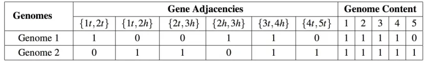
For example, gene 1 can be represented by {1h, 1t}. We used the gene ends and their

adjacencies to describe the permutations and positional relationships for all genes on the

chromosome. For instance, if gene 1 and gene 2 were adjacent, or gene −2 was followed

by gene −1 equivalently, these two genes can form a gene adjacency {1t, 2h}. A gene order

sequence {1, −2, 3, 4} can be labeled by a set of gene adjacencies: {1t, 2t}, {2h, 3h}, {3t,

4h}. In this paper, our algorithms further encoded genome content and gene adjacencies

into binary sequences for each chromosome. For instance, for two genomes with only one

chromosome, G1= {1, −2, 3, 4}, and G2 = {1, 2, 3, 4, −5}, we binary encode them as shown

in Table 2.1.

(25)

2.2.3 Improve MLWD for Yeasts Phylogenies Reconstruction

The previous MLWD method was restricted by its fixed evolutionary model and

the limitations in handling complex evolutionary events, such as deletion, duplication and

whole genome duplication. In this study, we will consider each single gene as the smallest

genome marker to process high-resolution genome datasets. First, we will statistically

analyze the evolutionary rates of different types of events for all species under the

Saccharomycetaceae family. Next, we will calculate the gene content and gene adjacencies

transition probabilities according to these genome evolutionary events.

Next, we will use these transition probabilities to build a constrained evolutionary

model based on the principle of double-cut-and-join (DCJ) operation (Friedberg, Darling,

& Yancopoulos, 2008; Yancopoulos, Attie, & Friedberg, 2005). This yeast evolutionary

model takes all kinds of genome level evolutionary events into account, including

rearrangements, insertions, deletions, and duplications. Based on the DCJ operation, each

event will always remove two old adjacencies randomly, and use the new ends to create

two new adjacencies. However, our yeast evolutionary model also considers that each

genome has n genes and n + O (C) adjacencies with constrained adjacency variations. There

are !"#$"_" % possible ends. The transition probability to lose an adjacency is estimated by

" (($)$*$+)

#$- (.) . The probability to gain a new adjacency is estimated by

(($)$*$+)

"#/_{$- (#)}. n and C

represent the total number of genes and chromosomes for a specific species. R, D, I and d

represent the estimated number of rearrangements, duplications, insertion, and deletion

events for this species based on the evolutionary rates of Saccharomycetaceae family. We

also applied their corresponding transition probabilities to the ancestral genome

reconstructions. After encoding the yeast genomes into binary sequences and computing

(26)

program RAxML with fast bootstrapping (Stamatakis, 2014) to reconstruct the yeast

phylogeny with overall maximum likelihood. The reconstructed phylogeny and the same

input genome data will be fed into the next stage PMAG for ancestral reconstruction. The

bootstrapping support value for each internal node and leaf on the phylogeny is considered

in three levels: strong support (bootstrap value > 90), medium support (bootstrap value

between 60 and 90), and weak support (bootstrap value < 60).

2.2.4 Improve PMAG for Yeast Ancestor Reconstruction

Most present computational ancestral reconstruction approaches can only process

simplified real data or simulated datasets with unique genome marker and limited types of

evolutionary events (Alekseyev & Pevzner, 2009; Feijão & Meidanis, 2009; Hu et al.,

2013; Ma, 2010; Perrin et al., 2015; Xu & Moret, 2011; Zheng & Sankoff, 2011). The

previous version of our PMAG approach also faced the same problems (Hu et al., 2014,

2013). In this study, we improved the algorithms of PMAG approach to process all kinds

of evolutionary events and high-resolution real genome data. Our improved approach was

based on Bayes theorem and probabilistic frameworks. It used the yeast genome transition

evolutionary model to compute the gene adjacencies of a specific ancestral genome for

each edge of the yeast phylogeny. We considered each gene as a basic genome marker and

reconstructed the ancestral genomes by maximizing the overall conditional probabilities of

ancestral marker sets along the edges of the phylogenetic tree.

First, we encoded genome content and gene adjacencies into binary sequences, as

shown in Table 2.1. The duplicated genes and adjacencies were encoded as additional

distinct elements and stored into an additional matrix. Furthermore, we computed the

conditional probabilities for all possible adjacencies across all genomes and assigned the

(27)

(from the phylogeny reconstruction step) as the guide tree, and assembled gene adjacencies

into ancestral genomes for all internal tree nodes with the maximum portability. For each

ancestral genome reconstruction, we re-rooted the tree and treated the ancestral genome

that needed to reconstruct as the new root and built the ancestral genome with the global

maximum probability over all species. We reconstructed gene orders of ancestral nodes by

using a similar idea from a previous probabilistic reconstruction approach for sequence

data (Yang, Kumar, & Nei, 1995). We also used the RAxML (Stamatakis, 2014) to estimate

evolutionary distance "d”. Our method iterated the steps above to compute all the

probabilities of adjacencies for each internal genome. Once all of these probabilities were

obtained, we converted this genome adjacencies assembly/reconstruction problem into an

instance of the Traveling Salesman Problem (TSP), and then used the

Chained-Lin-Kernighan heuristic TSP solver Linkern to solve this problem (Applegate, Bixby, Chvatal,

& Cook, 2006). The original yeasts input genomes were not well assembled. Many genome

contigs couldn’t be assembled or mapped back to regular chromosomes. Even though the

real yeast genome data suffered from these issues, the TSP solver helped us to better

assemble/reconstruct ancestor genomes by using all available adjacencies information in

known genomes. We mapped the gene content, gene adjacencies, and duplicated genes

information with the outputs from TSP solver. Finally, we determined the chromosome

structures of reconstructed ancestral genomes based on the chromosome structure

information from its parent and children genomes. We first identified all chromosome

telomeres for its parent and two children genomes. Next, we introduced the ancestral

chromosome telomeres with new chromosome telomeres by the following orders: 1,

telomeres shared by all three genomes (one parent and two children genomes); 2, shared

(28)

5 existed in one of children genomes. Finally, when the chromosome number reached the

number of its two children genome or its parent genome, we output the updated ancestral

genomes with correct chromosome number and chromosome telomeres.

2.3 YEAST PHYLOGENIES RECONSTRUCTION

2.3.1 phylogeny built from 11 yeast species.

We first used our improved computational approach MLWD (Method 3) to

construct the phylogeny for the first yeast genomes dataset with 11 species, which are

available in YGOB (Version 3 April 2009). Five of them are post-WGD species under four

genera. Six of them are non-WGD species under other four genera. This was the same

dataset that used in Gordon’s ancestor reconstruction study (Gordon et al., 2009). As shown

in Figure 2.1, we correctly classified all yeast species into their corresponding genera, and

also into their corresponding groups, post-WGD and non-WGD. We compared this

phylogeny with the recent studies and publications. First, we compared with the yeast

phylogeny from NCBI taxonomy (http://www.ncbi.nlm.nih.gov/taxonomy). Our

phylogeny was in accord with NCBI taxomony for all 11 species. Our phylogeny also

matches the phylogeny in Gordon’s ancestral reconstruction study (Gordon et al., 2009).

Recently, Salichos used a sequence alignment based maximum likelihood approach to

study the phylogeny of 23 yeast species by concatenation analysis of 1,070 orthologs

(Salichos & Rokas, 2013). Marcet-Houben and Vakirlis also used similar methods to infer

the phylogenies of 19 and 34 yeast species from shared orthologs and homologs

(Marcet-Houben & Gabaldón, 2015; Vakirlis et al., 2016). Even though our approach uses gene

order data and phylogenetic signals from genome level evolutionary events, our phylogeny

(29)

results with the NCBI taxonomy and recent publications demonstrate that our approach can

reconstruct very accurate phylogeny.

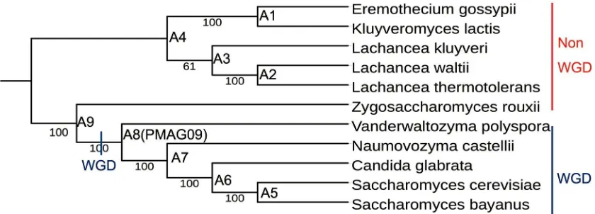
Figure 2. 1 Yeasts phylogeny built from all types of evolutionary events from 11 yeast species. Each leaf represents a species, and each internal node represents a common ancestor (A1 - A9). All internal edges have bootstrapping values of 100 except the branch between Lachancea genus and Eremothecium genus, which has a bootstrapping value of 61. The red line shows the non-WGD species, while the blue line shows the post-WGD species. We label A1 - A9 as the reconstructed yeast common ancestors built from the first yeast dataset. The ancestor A8 (PMAG09) shows the pre-duplication ancestor PMAG09, which is the step before yeasts’ WGD event in evolutionary.

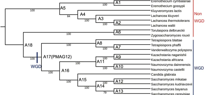
2.3.2 Yeasts phylogeny built from 20 yeast species.

We continued to construct the phylogeny for the second dataset with 20 species,

which are available in the latest version of YGOB (version 7 August 2012) (Byrne &

Wolfe, 2005; Gordon et al., 2011). Twelve of them are post-WGD species under six genera.

Eight of them are non-WGD species under other five genera. As shown in Figure 2.2, we

correctly classified these 20-yeast species into their corresponding genera, and also into

their corresponding groups, post-WGD and non-WGD. This phylogeny also entirely agrees

with the NCBI taxonomy. Although Salichos, Marcet-Houben, and Vakirlis performed

(30)

analyzing different gene datasets, their phylogenies still had conflicts between each other

(Marcet-Houben & Gabaldón, 2015; Salichos & Rokas, 2013; Vakirlis et al., 2016). Our

phylogeny agrees with Marcet-Houben’s phylongey on each of the shared 18 species,

except for the placement of K.lactis, which is still at the same evolutionary position in both

phylogenies. However, it is closer to the Lachancea genus in our phylogeny, while it is

closer to the Eremothecium genus in Marcet-Houben, Vakirlis, and Salichos’s phylogenies

(Marcet-Houben & Gabaldón, 2015; Salichos & Rokas, 2013; Vakirlis et al., 2016). We

could remove this small discrepancy by using the phylogenetic signals only from genome

rearrangement events. Our phylogeny agrees with Vakirlis’s phylogeny on their shared 20

species, only has two discrepancies. In our phylogeny, S. bayanus is a sibling of S.

cerevisiae, which agrees with Marcet-Houben (Marcet-Houben & Gabaldón, 2015). In

Vakirlis’s phylogeny, S. bayanus is the uncle of S.cerevisiae (Vakirlis et al., 2016), which

agrees with Salichos (Salichos & Rokas, 2013). For the placement of species N.castellii,

Marcet-Houben, Vakirlis, and our phylogeny agree with each other, while Salichos’s

phylogeny does not (Marcet-Houben & Gabaldón, 2015; Salichos & Rokas, 2013; Vakirlis

et al., 2016). Our phylogeny also agrees with Salichos’s phylogeny on their shared 13

species except for the differences noted above (Salichos & Rokas, 2013). The differences

may be caused by the inconsistencies in multiple sequence alignments and inaccuracies in

gene order annotations. For example, in the yeast genome database YGOB, some genes

cannot be mapped back to their corresponding chromosomes, which may cause inaccurate

adjacency information and result in misleading phylogenetic signals (Byrne & Wolfe,

2005).

The results above illustrate that our phylogenies are as accurate as those built from

(31)

using the gene order data and phylogenetic signals from genome level evolutionary events.

Our approach skips the multiple sequence alignment step and avoids the conflicting

phylogenetic signals from local and biased DNA sequences. We provide an independent

and alternative way to build the phylogenies for real genome datasets, and eliminate the

conflicting issues in traditional multiple sequence alignment based approaches.

(32)

2.4 YASET ANCESTRAL GENOME RECONSTRUCTIONS

2.4.1 Yeast Ancestral Genomes Reconstruction From 11 Yeast Species.

Recently, Wolfe reported that whole genome duplication (WGD) was found in the

common ancestor of six genera of Saccharomycetaceae family (Wolfe, 2015). Gordon

applied a parsimony-based approach to reconstruct the common ancestral genome dating

back to 100 million years ago, right before yeasts’ WGD event (Gordon et al., 2009).

Gordon used a sequence alignment-based phylogeny as the guide tree, and manually

reconstructed the gene orders of the ancestral genome from a dataset with 11 yeast species

(this also refers to the first yeast genome dataset in this study) (Byrne & Wolfe, 2005;

Gordon et al., 2009). The preliminary version of this manually reconstructed ancestral

genome was reported as a ‘gold standard’ in Sankoff’s studies (Gordon et al., 2009; Zheng,

Zhu, Adam, & Sankoff, 2008). In this paper, we use MANUAL09 to represent this version

of the manually reconstructed yeast ancestor. In 2012, Byrne and Wolfe added nine

additional yeast species to YGOB. They used the same method and reconstructed the

‘benchmark’ version ancestral genome, using genome information of 20 yeast species (this

also refers to the second yeast genome dataset) (Byrne & Wolfe, 2005; Gordon et al., 2011).

We use MANUAL12 to represent this ‘benchmark’ version ancestral genome. The

MANUAL12 ancestral genome was built from a dataset that contained more

comprehensive genome information of yeast species, indicating more accurate ancestral

reconstructions than the ancestor built from the first dataset (MANUAL09).

In this section, we first used our improved computational approach PMAG (the

fourth point of the Methods) to reconstruct the ancestral genomes for the first yeast genome

dataset. We used the phylogeny that reconstructed from the same input data in Figure 2.1

(33)

root ancestral genomes for these 11 yeast species. There are nine ancestral genomes

reconstructed and labeled as A1- A9 in the phylogeny of Figure 2.1. We have listed the

ancestral genome information in Supplementary dataset 1. Gene numbers of each ancestral

genome vary between 4,841 and 5,133. Each ancestral genome is represented by a list of

ancestral genes with their corresponding gene orders that shared across the whole

Saccharomycetaceae family. Among our reconstructed ancestors, we use PMAG09 (also

labeled as A8 in Figure 2.1) to represent our pre-WGD ancestor at the same evolutionary

stage with MANUAL09 and MANUAL12. Our first results comparison was among the

genome content of PMAG09, MANUAL09, and MANUAL12 ancestors, which contained

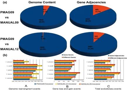
4,856, 4,703, and 4,943 genes, respectively. As Figure 2.3 (a) shows, the genome contents

of our PMAG09 ancestor are very similar to both MANUAL09 and MANUAL12. Of all

the genes in PMAG09, 4,645 (95.6%) are shared by MANUAL09, and 4,836 (99.6%) are

shared by MANUAL12. We also compared all gene adjacencies among these three

ancestral genomes, which could reflect the absolute differences of gene contents,

directions, and permutations between any two genomes. Figure 2.3 (a) shows that our

ancestor PMAG09 shares 4,192 (86.3%) gene adjacencies with MANUAL09, and 4,464

(91.9%) gene adjacencies with MANUAL12.

We identified all gene pairs (gene adjacencies) that never split during evolution,

which were called “non-split adjacencies”. There were 697 “non-split adjacencies” shared

by the descendant genomes of PMAG09 and MANUAL09, and 269 “non-split

adjacencies” shared by the descendant genomes of MANUAL12. in our reconstructed

ancestral genomes, PMAG09 contained 638 (13.1%) “non-split adjacencies”.

MANUAL09 contained 609 (12.9%) “non-split adjacencies”. MANUAL12 contained 253

(34)

shared 3,554 (84.2%) adjacencies with MANUAL09 and 4,211 (91.4%) adjacencies with

the “benchmark ancestral genome” MANUAL12. We further identified and compared the

number of different types of evolutionary events between the automated/manually

reconstructed ancestors and their shared five present post-WGD descendant genomes. We

applied a computational method to calculate genome evolutionary events based on the

principle of double-cut-and-join (DCJ) operation (Friedberg et al., 2008; Yancopoulos et

al., 2005), which could identify all events that occurred during evolutionary history. Under

DCJ operation model, if we had identified n evolutionary events between genome A and

Genome B, the gene order permutations could evolve from genome A to genome B by

these n events. Figure 2.3 (b) A shows that our ancestor PAMG09 presents the least number

of genome rearrangement events when compared with MANUAL09 and MANUAL12.

Figure 2.3 (b) B shows a similar result for gene loss and gain events. Likewise, Figure 2.3

(b) C shows that our ancestor PMAG09 has the least number of overall evolutionary events

among these three ancestors.

These results demonstrate that our ancestor PMAG09 is very similar to both

manually reconstructed ancestral genomes in genome content and gene adjacencies.

Although our ancestor PMAG09 is reconstructed from the same data as the old version

ancestor MANUAL09, it is more similar to the “benchmark” ancestor MANUAL12.

MANUAL12 is built from the second dataset with more comprehensive genome

information of nine additional yeast species, which indicates more accurate ancestral

reconstructions. Moreover, PMAG09 has fewer evolutionary events than both

MANUAL09 and MANUAL12. Therefore, PMAG09 is more optimal and parsimonious

ancestral genome than both manually reconstructed ancestral genomes from an

(35)

Figure 2. 3 Genome content, gene adjacency and evolutionary events comparisons among PMAG09, MANUAL09, and MANUAL12 ancestors. Figure (a), Genome content and gene adjacency comparisons among PMAG09, MANUAL09, and MANUAL12 ancestors. (b), Evolutionary events comparisons among the evolutionary histories of PMAG09, MANUAL09, and MANUAL12 ancestors. Figure (b) A, B and C show the total number of genome rearrangements events, gene loss and gain events, as well as overall evolutionary events between ancestral genomes and their shared five present post-WGD descendants.

2.4.2 Yeast Ancestral Genomes Reconstruction from 20 Yeast Species.

We further reconstructed the ancestral genomes for the second yeast genome

dataset with 20 species. We used the phylogeny reconstructed from the same input data in

Figure 2.2 as the guide tree and reconstructed the ancestral genomes within 55 minutes.

There are 18 ancestral genomes reconstructed and labeled as A1 - A18 in the phylogeny of

(36)

listed the ancestral genes for each ancestor and analyzed their functions in Supplementary

Dataset 2. Among the 18 ancestral genomes reconstructed here, we used PMAG12 (also

labeled as A17 in Figure 2.2) to represent the pre-WGD ancestor at the same evolutionary

step with MANUAL12. The post-WGD ancestor A17’ had an additional copy of pre-WGD

ancestor A17. Therefore, it had the same gene orders and genome information as pre-WGD

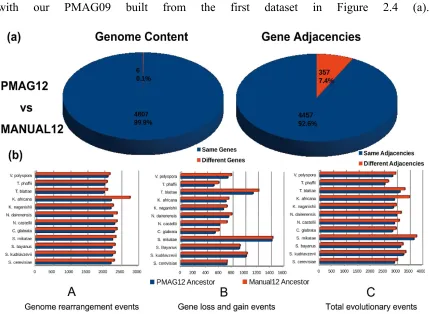
ancestor A17. There are 4,813 genes in PMAG12 and 4,943 genes in MANUAL12. As

Figure 2.4 (a) shows, these two ancestors are extremely similar. PMAG12 shares 4,807

(99.9%) of its genes and 4,457 (92.6%) of its gene adjacencies with MANUAL12.

We compared different reconstructions on the proportions of adjacencies that were

split during evolution. There were 269 “non-split adjacencies” shared by the descendant

genomes of PMAG12 and MANUAL12. In our reconstructed ancestral genomes,

PMAG12 contained 258 (5.3%) “non-split adjacencies”. MANUAL12 contained 253

(5.1%) “non-split adjacencies”. After removing all “non-split adjacencies”, PMAG12 still

shared 4,199 (92.1%) adjacencies with the “benchmark ancestral genome” MANUAL12.

We continued to compare the number of different types of evolutionary events between

ancestors and their 12 descendants. As Figure 2.3 (b) shows, even though PMAG12 and

MANUAL12 are built from the same dataset, PAMG12 has fewer genome rearrangements,

fewer gene losses and gains, and fewer total evolutionary events than MANUAL12 in their

evolutionary history.

These results also illustrate that our ancestors are very similar to the manually

reconstructed ancestors in genome content and gene adjacencies. Furthermore, our

ancestors provide us with more optimal and parsimonious solutions from an evolutionary

perspective, because our automated approach searches for globally optimal gene

(37)

approach only scans a fixed number of genes, and visually compares these gene orders

(Byrne & Wolfe, 2005; Gordon et al., 2011, 2009). Therefore, the manual ancestral

genomes might be restricted in a local view of gene adjacency and content, and reach a

solution with a set of local optimums. Moreover, as we expected, Figure 2.4 (a) shows that

PMAG12 is more similar to the latest ‘benchmark’ ancestor MANUAL12 when compared

with our PMAG09 built from the first dataset in Figure 2.4 (a).

(38)

2.5 ANCESTRAL GENOME RECONSTRUCTION ON SIMULATED DATA

To explore the performance of these ancestral reconstruction approaches, we select

four most famous and powerful approaches from both distance/event-based and

homology/adjacency-based categories. We analyze and compare their performance on

simulated datasets and evaluate their outputs. For the distance/event-based approaches, we

select MGRA2 and GASTS. MGRA2 is the only distance/event-based approach that could

deal with all kinds of evolutionary events (Avdeyev et al., 2016). GASTS is famous for its

speed and accuracy for small-scale datasets, but it could only handle the problems with

equal genome content (Xu & Moret, 2011). For the homology/adjacency-based

approaches, we select our method PMAG and Gapped Adjacency (Gagnon et al., 2012).

In order to compare the performances in unequal content genome datasets with more

complicated genome evolutionary events, we set up evolutionary events between any two

generations with 80% inversions, 10% translocations, 5% insertions and 5% deletions. The

settings for the evolutionary rates and genome sizes are the same.

Figure 2.2 presents the results analyses and comparisons for these four approaches.

For the distance/event-based approaches, GASTS could not handle these complicated

evolutionary events. MGRA2 was reported being capable of handling this kind of problem

(reference) but was not able to give any output after running for 48 hours for any of these

datasets. Only the homology/adjacency-based approaches could solve these problems and

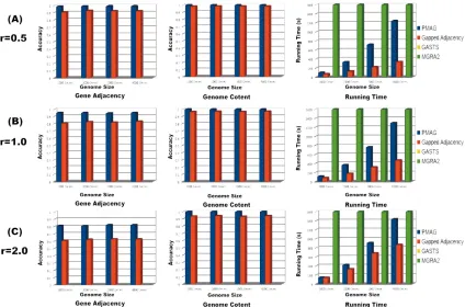
reconstruct the ancestral genomes. As it shown in Figure 2.5 (A), PMAG preserve very

high gene adjacency accuracy (almost 1.0) for all four datasets with different genome size,

while the accuracy of Gapped Adjacency is always about 10% lower (around 0.9) than

PMAG. Both PMAG and Gapped Adjacency could reconstruct the genome contents with

(39)

(around 0.95) in the genome content reconstruction. Gapped Adjacency requires less

running time than PMAG. Figure 2.5 (B) shows, when the evolutionary rate reaches 1,

PMAG could still keep a high accuracy (around 0.95), while Gapped Adjacency could only

reach the accuracy of 0.8. In the genome content and running time comparison, they have

the similar result with Figure 2.5 (A). Figure 2.5 (C) shows the performance of these

approaches under high evolutionary rate r=2. In this experiment, PMAG can still grantee a

sound gene adjacency accuracy of 0.8 for all four genome datasets. However, the Gapped

Adjacency can only reach the accuracy of 0.6. PMAG also maintains higher accuracy (>

0.95) than Gapped Adjacency (around 0.9) in the genome content reconstruction.

Compared with the three experiments above, PMAG outperforms Gapped

Adjacency in reconstructing the ancestral genome adjacency and genome content. PMAG

preserves consistently better performance than the Gapped Adjacency in all cases. As the

evolutionary rate getting higher, the accuracy gets lower, but PMAG could still keep a high

accuracy even the evolutionary rate is high. Both PMAG and Gapped Adjacency can

maintain very high accuracy in reconstructing the genome content. Both of them only

require hundreds of seconds to get the solutions for the small-scale or large-scale dataset.

The genome size of the testing dataset also has little influence on the performance of

accuracy for gene adjacency and genome content, but it did affect the running time. Gapped

Adjacency requires less running time than the PMAG in all experiments. MGRA2 cannot

(40)

Figure 2. 5 Results analyses and comparisons of different approaches on simulated genome datasets. The legend of MGRA2 is missing in this figure, because it cannot give any output after running for 48 hours. The legend of GASTS is missing in this figure, because it cannot handle these datasets.

2.6 SYNTENIC BLOCK AND THEIR GENE ONTOLOGY ANALYSIS

2.6.1 Evolutionary and Syntenic Block Comparisons among Reconstructed Ancestors

Comparisons analyses of syntenic blocks between genomes are powerful

approaches to study genomic evolution, gene origin, and gene co-evolution (Bhutkar et al.,

2008; Sankoff, 2009). In this study, we followed the above rules to define the syntenic

blocks, which was the genomic regions that contain two or more genes, maintaining the

same gene order and orientation (Ghiurcuta & Moret, 2014). We ran whole genome

comparisons among our automated reconstructed ancestors and manually reconstructed

(41)

Supplementary Dataset 3. As Table 2.2 shows, PMAG09 shares 337 syntenic blocks with

MANUAL09, which contains 4553 (93.7%) syntenic genes. PMAG09 shares 256 syntenic

blocks with MANUAL12, which contains 4753 (94.2%) syntenic genes. Although both

PMAG09 and MANUAL09 are reconstructed from the same dataset, PMAG09 is more

similar to MANUAL12 in genome contents and chromosome sub-structures (shares more

syntenic genes, less syntenic blocks, and longer syntenic block lengths). Table 2.2 also

shows that PMAG12 shares 233 syntenic blocks with MANUAL12, which contains 4733

(93.7%) syntenic genes. PMAG12 has the highest similarity with MANUAL12 in genome

contents and sub-structures when compared with MANUAL09 and PMAG09. We also

draw the chromosome dot plots between our ancestors and the "benchmark" ancestor

MANUAL12, which could illustrate the level of colinearity between them. As the Figure

2.6 (a) and (b) shown, our reconstructed ancestral genome PMAG09 and PMAG12 have

good chromosome colinearity with the “benchmark” ancestral genome MANUAL12,

which illustrated that they shared many same chromosome sub-structures. In addition,

Figure 2.6 (b) also illustrates that our PMAG12 ancestor has better chromosome colinearity

with the "benchmark" ancestral genome MANUAL12 when compared with PMAG09.

As we expected, our ancestor PMAG09 and PMAG12 was more consistent with

the latest ’benchmark’ ancestor MANUAL12 in genome contents and structures than

ancestor MANUAL09, which was built from the first dataset. Furthermore, our PMAG12

ancestor was more consistent with MANUAL12 than our PMAG09 ancestor, since the

reconstruction of PMAG12 uses additional information. The results above are also

consistent with the results that we obtained in the ancestral genome dot plots in Figure 2.6,

as well as the results in the ancestor genome contents and gene adjacencies comparisons in

(42)

Table 2. 2 Syntenic genes and blocks among ancestral genomes.

Figure 2. 6 Chromosome dot plots between our ancestors and the "benchmark" ancestor MANUAL12. The eight y-axes of eight sub-figures showed the eight chromosomes of MANUAL12. The x-axes of each sub-figures represented all eight chromosomes of our ancestors.

2.6.2 Gene Function and Ontology Analyses of Syntenic Blocks

Next, we continued to run whole genome comparisons between all

automated/manually reconstructed ancestral genomes and their five present post-WGD

descendants to identify their shared conserved syntenic blocks. Table 2.3 shows that both

PMAG09 and PMAG12 share more syntenic genes with the present yeast species than

MANUAL09 and MANUAL12 do. They also preserve less syntenic blocks and longer

(43)

our ancestors PMAG09 and PMAG12 share more genome contents and sub-structures with

the present yeast species when compared with manually reconstructed ancestors. These

results also illustrate that our automated reconstructed ancestors are more optimal and

parsimonious genomes than manually reconstructed ancestors from an evolutionary

perspective, which also agrees with our previous results in Figure 2.3 (b) and Figure 2.4

(b). Furthermore, we annotated the genes and analyzed their functions for each syntenic

blocks among automated/manually reconstructed ancestors and present yeast species. This

information is critical to locate conserved co-evolution genes and functional gene groups

that exist in both ancestral and present species. It can be used to discover the correlations

between genome level structural and functional variations in yeasts’ evolutionary history.

For example, there are only a total of six genes in overall 7,165 genes associated with the

nucleotide salvage process in S.cerevisiae. The syntenic block No.2 shared by PMAG12

contains two of them in total eight genes (YDR399W and YDR400W), which has the

p-value of 0.002 in the gene ontology analysis. These results indicate that YDR399W and

YDR400W are conserved co-evolution genes to maintain their structural and functional

relationships in evolutionary processes.

Our approach uses a new evolutionary model that can process the real whole

genome data, non-identical content data, and all types of complex evolutionary events. This

model is based on the principle of double-cut-and-join (DCJ) operations and incorporates

the evolutionary rates of the Saccharomycetaceae family. It can be extended to other

multiple chromosome species after we encode all existing genes into gene orders and

(44)

Table 2. 3 Syntenic genes and blocks between ancestral genomes and present yeast genomes

2.7 DISCUSSION

Initially, studies of yeast phylogenies were based on morphological phenotypes and

characters such as sexual states, germinations, and fermentations (Kurtzman et al., 2011).

Currently, widely accepted yeasts phylogenetic approaches are based on multiple sequence

alignment. However, they still have limitations and often have conflicting results with each

other (Hedtke et al., 2006; Marcet-Houben & Gabaldón, 2015; Salichos & Rokas, 2013;

Vakirlis et al., 2016). In this study, we reconstructed the phylogenies for two

high-resolution yeasts genome datasets by using the phylogenetic signals from genome level

evolutionary events. The comparisons with the NCBI taxonomy and recent publications

demonstrated that our approach could also reconstruct very accurate and robust

phylogenies. We provide a new and alternative method to resolve the same phylogenetic

problems but using different types of data and phylogenetic signals. Our approach

considers each gene as a single marker and uses 14,101 total markers. Therefore, it will not

miss the phylogenetic signals from small-scale evolutionary events. It skips the multiple

sequence alignment step and avoids conflicting phylogenetic signals from distinct

molecular sequences in traditional phylogenetic approaches. Therefore, our approach can

eliminate the conflicting issues that exist in current multiple sequence alignment-based

phylogenetic approaches. Current whole genome level phylogenetic studies on real data

(45)

datasets(Figueroa & Baco, 2015; Weigert et al., 2016). However, our approach uses a new

evolutionary model that can process the real whole genome data, non-identical content

data, and all types of complex evolutionary events. This model is based on the principle of

double-cut-and-join (DCJ) operations and incorporates the evolutionary rates of the

Saccharomycetaceae family. It can be extended to other multiple chromosome species after

encoding all existing genes into gene orders and marking out all possible homologous

genes that shared by more than one genome.

Reconstructing ancestral genomes offers opportunities to study the evolutionary

mechanisms and trajectories of present species. Studies that focused on developing

computational ancestor reconstruction approaches face many difficulties. Present

computational approaches suffer from issues of simplistic evolutionary models, complex

datasets, and complex evolutionary events (Feng et al., 2017; Gao et al., 2015; Ma, 2010;

Perrin et al., 2015; Sankoff, 2009; Xu & Moret, 2011; L. Zhou et al., 2016). Recent studies

of Vakirlis’ et al. have made great achievements in computational ancestral reconstruction

approaches. The newly sequenced ten yeast species in the Lachancea genus and used

software AnChro to reconstruct the ancestral genomes on the Lachancea genus level

(Vakirlis et al., 2016). They used SynChro to identify conserved syntenic blocks based on

the DNA sequence information and additional parameters (Drillon, Carbone, & Fischer,

2014). They used ReChro to identify cycles of breakpoints for each pairwise combination

of genomes (Drillon, Carbone, & Fischer, 2011). They provided a granular view of genome

evolution within an entire eukaryotic genus (Vakirlis et al., 2016). In this study, we built

an automated pipeline to reconstruct phylogenies and ancestral genomes from whole

genome data. First, we built the phylogenies and then used them as guide trees to