SU(2) decomposition for the quantum information dynamics in 2 d-partite two-level quantum systems

SU(2) decomposition for the quantum information

dynamics in 2d-partite two-level quantum systems

Francisco Delgado1,† ID

1 _{Escuela de Ingeniería y Ciencias, Tecnológico de Monterrey; [email protected]}

† Current address: Departamento de Física y Matemáticas, Tecnológico de Monterrey, Campus Estado de México, Atizapán, Estado de México, México

Abstract:Quantum Computation, in the gate array version, uses logical gates adopting convenient forms for computational algorithms based on those of classical computation. There, two-level quantum systems are the basic elements connecting the binary nature of classical computation with the settlement of quantum processing. Despite, their design depends on specific quantum systems and physical interactions involved, exacerbating the dynamics analysis. Predictable and controllable manipulation should be addressed to control the quantum states, but resources are restricted to limitations imposed by the physical settlement. This work presents a formalism to decompose the quantum information dynamics in SU(22d)for 2d-partite two-level systems into 22d−1SU(2)quantum subsystems. Decomposition lets to set control procedures, to generate large entangled states and to design specialized dedicated quantum gates. There, easy and traditional operations proposed by quantum computation are recovered for more complex and large systems. Alternating the parameters of local and non-local interactions, the procedure states a universal exchange semantics on the generalized Bell states basis. It could be understood as a momentary splitting of the 2dinformation channels into 22d−1_{pairs of 2 level quantum information subsystems}

and a settlement of the quantum information manipulation free of the imposed restrictions by the underlying physical system.

Keywords:Quantum information; Quantum dynamics; Entanglement

1. Introduction

Quantum Information is generating new applications and tentative future technologies as Quantum Computation [1–3] and Quantum Cryptography [4,5] based on disruptive phenomena. In this arena, understanding of quantum information dynamics and control of quantum systems is a compulsory development to manage the quantum resources involved. Applications require a tight control of resources and interactions, in particular those related with coherence and entanglement, which are fundamental in the most of applications. Thus, Quantum Control has developed fine management of physical variables to prepare, maintain and transform quantum states in order to exploit them for concrete purposes. The outstanding high-tech commercial appliances as D-Wave and IBM-Q use qubits in the form of two-level systems, whatever superconducting circuits or ions as well as several approaches to their interconnecting architecture.

For multipartite systems, research in control is oriented to achieve different goals involved in quantum applications. The most of them are numerical approaches more than analytical due to the inherited complexity in the quantum information dynamics when the number of parts grows. For a single system with a two-level spectrum, the control problem has been extensively studied in terms of exact optimal control for energy or time cost [6,7]. Recently, research for the anisotropic Heisenberg-Ising model for bipartite systems inSU(4)[8] has shown how this model exhibitsSU(2) block decomposition when it is written in the non-local basis of Bell states instead of the traditional computational basis. It means thatH2_{becomes a direct sum of two subspaces, each one generated}

by a pair of Bell states, whileUunderlies in the semi-direct productU(1)×SU(2)2_{. Thus, control}

can be reduced to twoSU(2)control problems in each block and exact solutions for some control procedures can be found [9,10]. There, controlled blocks can be selected by the direction of external driven interactions introduced. That scheme lets controlled transformations between Bell states on demand and therefore on general states. Thus, the procedure sets a method of control to manipulate quantum information on magnetic systems where computational grammar is based on Bell states instead of traditional computational basis, letting an easier programmed transformation among any pair of elements in that basis. This result become an inspiration to reproduce similar decomposition schemes for larger systems in terms of simpler problems based on quasi-isolated two-level subsystems, stating easier and universal (not necessarily optimal) controlled manipulation procedures for quantum information. Technology to set up the possible architecture of these generic systems is being currently achieved through trapped-ion qubits [11] and superconducting qubits [12].

Thus, the generalization ofSU(2)block decomposition is a formalism to express the dynamics in a convenient basis revealing certain quantum information states algebraically free of the most of complexity introduced by the entangling operations (which does few convenient the use of computational basis based on eigenstates from single systems before the entangling interactions) but still conserving their entangled properties. It reveals how the probability exchange happens together with the structure of entanglement behind of randomness introduced by the complexity for large quantum information systems. Still, as for their predecessor, those basis maintain certain degree of universality including several alternative local and non-local interactions, which as for their SU(4)predecessor, when they are combined state a series of punctual operations able to set: a) fine control based on well knownSU(2)control procedures, b) construction of universal gates for the entire process based on two-channel like operations, and c) design of more complex dedicated multi-channel gates by factorization.

The general aim of this paper is demonstrate that such decomposition and reduction is achievable for large qubit systems more than those in [8,10]. The second section states the general Hamiltonian to be analyzed. The third section shows how theSU(2)decomposition procedure can be generalized on a general n-partite two-level systems (not only for the driven Heisenberg-Ising interactions), reducing them to 2n−1selectable transformations between pairs of specific quantum states. Then, these transformations could be based on known control schemes forSU(2)systems as those in [6,7]. The selection of these 2n−1pairs of states has room to be settled on convenience of the quantum process being considered and the resources involved. Thus, the basis on which the decomposition can be established works as a computational grammar for the quantum procedures being attained. These basis are not completely arbitrary, thus, the fourth section shows how a kind of Bell basis generalization is able to generate theSU(2)decomposition for an even number of parts,n = 2d. Then, the fifth section is devoted to analyze the restrictions on the Hamiltonian to get theSU(2)decomposition, the inherited states and the block properties. This analysis includes a classification of interactions able to generate theSU(2)decomposition. Due to the procedure being presented could reproduce complex quantum gates, generate large entangled states and introduce control procedures inSU(22d)when the grammar is based on the proposed generalized Bell states, the sixth section analyzes potential applications in these trends. The final section concludes summarizing the findings and settling the related future work to be developed.

2. Generalized Hamiltonian

The problem can be established for a general Hamiltonian forncoupled two-level systems on U(2n)conforming a closed system. It can be written as a general combination of tensor products of Pauli matrices for each subsystem:

˜ H=

∑

{ik}

h{i_k} n O k=1

σi_k =

4n₋₁

∑

hIn

4 n O k=1

σIn

where {ik} = {i1,i2, . . . ,in}, ik = 0, 1, 2, 3 and h{i_k} is a set of time dependent real functions in general. Sometimes, as in the second expression in (1), {ik} will be represented as the number

I ∈ {0, 1, . . . , 4n−1}as it is expressed in base-4 withndigits,In

4. Then,I4,nk =ikfork=1, 2, . . . ,n. σikforik=0, 1, 2, 3 are the traditional Pauli matrices in the computational basis|0i,|1i ∈ H

2_{for each}

partk. Note that due toSU(2)algebra of Pauli matrices, this Hamiltonian comprises all analytical Hamiltonians based on two-level systems with nparts. The Hamiltonian obeys the Schrödinger equation for its associated evolution operator ˜U:

˜

HU˜ =ih¯∂U˜

∂t (2)

Despiteh{0,...,0}is not necessarily zero, if{E˜j|j= 1, . . . , 2n}are the eigenvalues of ˜HandE ≡

∑2n

j=1E˜j=2nh{0,...,0}, then defining:

H≡_H˜ −h{0,...,0} n O k=1

σ0, U≡Ue˜ i

¯

hh{0,...,0}t ₍₃₎

these operators become the equivalent traceless Hamiltonian and its corresponding evolution operator with eigenvaluesEj=E˜j−h{0,...,0}, both fulfilling (2) too. Hand ˜Hhave the same set of eigenvectors

{ b_j

∈ H2n_{|j=1, . . . , 2}n_{}. Thus, the Hamiltonian can be written alternatively asH=∑}2n

j=1Ej b_j b_j

. Thus, in the following, the Hamiltonian could be assumed traceless without lost of generality. Note while ˜U∈U(2n), thenU∈SU(2n). In the further development onlyHandUsymbols will be used as equivalent to ˜Hand ˜U.Hcan be split in two parts, the localHland the non-localHnlinteractions:

Hl=

n

∑

3

∑

h_(i4k−1₎n

4 n O s=1

σ_(i4k−1₎n

4,s →

˜

H=H˜nl+Hl (4)

where(i4k−1)₄nis the numberi4k−1represented in base-4 withndigits and(i4k−1)n_4,sis itssthterm in that base.

3. SU(2) decomposition generalities

TheSU(2)decomposition procedure, as it was found in [8], can be induced by considering a set of 2n orthogonal states: {|αii}and 2n−1pairs{j(i),k(i)},i = 1, 2, ..., 2n−1withk(i) = j(i) +1∈

{2, 4, ..., 2n}related with the eigenvalues through a mixing matrix, in such way that they fulfill:

|b2i−1i=Ai αj(i)

E +Bi

αk(i)

E

→

αj(i) E

= A∗_i |b2i−1i −Bie−iφ|b2ii

|b2ii=−B∗ieiφ αj(i)

E

+A∗_ieiφ αk(i)

E

→

αk(i) E

=B_i∗|b2i−1i+Aie−iφ|b2ii (5) with:|Ai|2+|Bi|2=1, where last relations are clearly true because orthogonality (note that energies Ejbecome ordered as the states are paired). States{

α_j

}are then defined by theAi,Biselection. Each pair sets one of the orthogonal subspaces:

H2_i =span({|b2i−1i,|b2ii}) =span({ αj(i)

E ,

αk(i) E

})→ H2n =

2n−1

M i=1

There are lots of possibilities for this selection, but not necessarily all practical basis fit in this construction. In particular, separability or entanglement properties are not necessarily assured for

{|αii} as in [8]. Clearly, because these states are assumed unitary, then Ai = D

b2i|αk(i)

E eiφ ₌ D

b2i−1|α_j(i) E∗

,Bi = D

b2i−1|α_k(i) E∗

= −Db2i|α_j(i) E

eiφ_{. By applyingH on (5) and considering that}

|biihas the eigenvalueEi, it is possible arrive to the following expressions:

H αj(i)

E

= (|Ai|2E2i−1+|Bi|2E2i) αj(i)

E

+A∗_iBi(E2i−1−E2i) αk(i)

E

H αk(i)

E

= AiB∗i(E2i−1−E2i) αj(i)

E

+ (|Ai|2E2i+|Bi|2E2i−1)

αk(i)

E

(7)

which gives the Hamiltonian components in this basis:

D

αj(i)|H|αj(i)

E

= |Ai|2E2i−1+|Bi|2E2i D

α_k(i)|H|α_k(i) E

= |Ai|2E2i+|Bi|2E2i−1

D

α_j(i)|H|α_k(i) E

= AiB∗i(E2i−1−E2i) (8) which can be alternatively obtained from (5). Note that phase φ is non-physical. This basis transformation changes the diagonal structure for the basis{|bii}into a 2×2 diagonal block structure for the basis{

α_j

}. For simplicity, we define the following quantities:

Ai =rAie

iγ_Ai

,Bi=rBie

iγ_Bi

∆±

i = 2¯1h(E2i±E2i−1)

Γi=γA_i−γBi (9)

then, each 2×2 block inH, labeled asSH i, can be written in matrix form as:

SH i = ∆

+

i −(rAi

2_−r

B_i2)∆−_i −2rAirBi∆ − i eiΓi

−2rAirBi∆ −

i e−iΓi ∆+i + (rAi

2_−r

Bi 2_)∆−

i !

= ∆+_{i Ii}−2rAirBi∆ −

i cosΓiXi+2rAirBi∆ −

i sinΓiYi−(rAi

2_−r

Bi 2_)∆−

i Zi (10)

≡ ∆+

i Ii+SH0i (11)

where despiterAi

2_+r

Bi

2_{=1, we use both termsr}

Ai andrBi for the symmetry. In addition,Ii,Xi,Yi

andZiare respectively the 2×2 unitary matrix and the Pauli matrices settled for the blockSH i. Thus, Hcan be written as a sum of operators acting on the different subspacesH2

i or as the following direct sum structure of 2n−12×2 block-diagonal matrices:

H =

2n−1 O i=1

SH i=      

SH1 0 . . . 0

0 SH2 . . . 0

..

. ... . .. ... 0 0 . . . SH2n−1

      (12)

with 0, the 2×2 zero matrix. Because this structure is preserved under matrix products, it is inherited by the evolution matrixU. In particular, if Hamiltonian (1) is not time dependent, then U=∑2_j=n₁e−hi¯Ejt_b

j bj

SU i = e−

i

¯

hE2i−1t_|b

2i−1i hb2i−1|+e− i

¯

hE2it_|b

2ii hb2i|= = e−i∆+i t

(ei∆−i t−_2irB i

2_sin∆−

i t)

α_j(i) α_j(i) + 2irAirBisin∆

− i t(e

iΓi_α

j(i)hαk(i)|+e−iΓi|αk(i)iαj(i) ) + (e−i∆−i t+2ir_B

i

2_sin∆−

i t)|αk(i)i hαk(i)|

(13)

similarly, in matrix form or in terms ofIi,Xi,YiandZi:

SU i = e−i∆ +

i t cos∆ −

i t+i(rAi

2_−r

Bi

2_)sin∆−

i t 2irAirBie

iΓi_sin∆−

i t 2irAirBie

−iΓi_sin∆−

i t cos∆

−

i t−i(rAi

2_−r

Bi

2_)sin∆−

i t !

= e−i∆+i t

cos∆−_i tIi+2irAirBicosΓisin∆ − i tXi− 2irAirBisinΓisin∆

−

i tYi+i(rAi

2_−r

Bi

2_)sin∆−

i tZi

(14)

note that the election ofΓilets simplify last expression to contain only one operator betweenXiandYi (as in [8,9]). This property is useful for the optimal control in each block based on the prescriptions in [6]. Then, similarly asH:

U =

2n−1

O i=1

SU i =      

SU1 0 . . . 0

0 SU2 . . . 0

..

. ... . .. ... 0 0 . . . SU2n−1

      (15)

where in general for the time-dependent Hamiltonian:

SU i = τ{e− i

¯

h Rt

0SH i_dt0_}=e−i∆+i t_τ{_e−¯hi Rt

0SH0i_dt0} ₍₁₆₎

being τ, the time ordered integral. It implies that U is an element in the semi-direct product

U(1)2n−1−1×SU(2)2n−1 ⊂SU(2n)(due to any factor phasee−i∆+i tdepends on the remaining phase

factors through E). In the following, informally, we will call to this factorization as the SU(2) decomposition (in reality, each block has the formU(1)×SU(2)), due to the block structure. As a consequence, Hilbert spaceHn_{becomes the direct sum of 2}n−1_{subspaces generated by each pair} {

αj(i) E

, αk(i)

E

}, i = 1, 2, . . . , 2n−1. In each subspace, the dynamics mixes the probabilities, but probabilities among subspaces remain unmixed while there are not an rearrangement in the pairing between{|bii}and{

α_j

}(clearly, in this rearrangement the basis{ α_j

}could change). Thus, if

|ψ0i = ∑2 n−1

i=1 |ψ0ii is the initial state with |ψ0ii = ψ0i,j(i)

αj(i)

E

+ψ0i,k(i)

αk(i)

E

, then its evolved

component in the subspacei=1, 2, ..., 2n−1fulfillsk |ψ_tii k=kSU0i |ψ0ii k=k |ψ0ii k.

4. GBS: a non-local basis fitting in {αj

}

Non-local basis are been used as theoretical resource to show explicitly how evolution [13] and measurement [14] could generate entangled states. In [8] was shown that Heisenberg-Ising model including driven magnetic fields in a fix direction lets to generate the block structure depicted there for the traditional Bell basis. Thus, the Bell basis for two-level bipartite systems has shown fit in the U(1)×SU(2)2_{decomposition ofSU(4). Despite the added complexity to manage non-local states,}

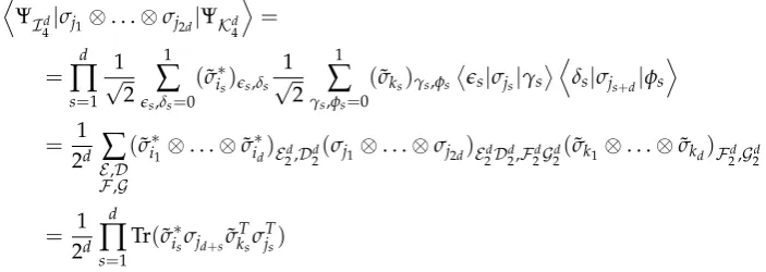
recent work goes in that direction, the control of entangled states [15]. This basis works as a universal basis for the Heisenberg-Ising interaction including an external magnetic field in any specific direction on a couple of qubits [8–10]. This model includes other interactions models asXXX[16] ,XY[17] andXXZ[18]. In the current development, the most obvious guess is the Generalized Bell States (GBS) basis forn=2dpresented in [19] as tensor products of Bell states. In the next sections some further useful formulas are obtained to show then how GBS basis fits inSU(2)decomposition for larger systems than bipartite ones.

4.1. GBS basis and Hamiltonian components

Forn=2d, GBS basis [19] forms an orthogonal basis of partial entangled states for 2dparticles. Each element in such basis can be written in a brief way as:

ΨI₄d

E =

d O s=1

1

√

2

1

∑

(σ˜is)es,δs|esδsi (17)

= √1

2d

∑

(σ˜i1⊗. . .⊗σ˜id)e1...ed,δ1...δd|e1. . .edi ⊗ |δ1. . .δdi (18)

= √1

2d

2d−1

∑

(σ˜i1⊗. . .⊗σ˜id)E₂d,Dd

2 E

d

2

E

⊗

D d

2

E

(19)

where{ej} = {e1, . . . ,ed},{δk} = {δ1, . . . ,δd};ej,δk = 0, 1. At this point, ˜σi can be considered as proportional unitaries to the traditional Pauli matrices [19]. In addition,Id

4 is a brief expression of {i1,i2, . . . ,id}as the digits set ofI ∈ {0, 1, . . . , 4d−1}when it is written in base-4 withddigits. In a similar way,Ed

2,D2dare numbers written in base-2 withddigits (E,D ∈ {0, 1, . . . , 2d−1})representing {e1, . . . ,ed},{δ1, . . . ,δd}respectively (be aware about the fact that digits are reversed as commonly they appear inEd

2 orI4dexpressions). In the following, for simplicity, we useIbdandI indistinctly, the basebcould be normally inferred from the context. Each element in this basis is not maximally entangled, instead they have maximally entangled bipartite subsystems, which are separable from the remaining system. Separable pairs contain the parts[s,s+d],s=1, 2, ...,d(in the following, square brackets will be used to point out a subsystem of parts in the whole system).

In order{ ΨI₄d

E

}(I ∈ {0, 1, . . . , 4d−1}) reaches the kind of sets{ αj

D

ΨId

4|σj1⊗. . .⊗σj2d|ΨK4d E

= =

d

∏

1

√

2

1

∑

(σ˜_i∗_s)_es,δs

1

√

2

1

∑

(σ˜ks)γs,φs

es|σjs|γs

D

δs|σj_s+d|φs

E

= 1 2d

∑

E,D F,G

(σ˜_i∗

1⊗. . .⊗σ˜

∗

id)E₂d,Dd₂(σj1⊗. . .⊗σj2d)E₂dDd₂,Fd

2G2d(σ˜k1⊗. . .⊗σ˜kd)F2d,G2d

= 1 2d

d

∏

Tr(σ˜_i∗_sσjd+sσ˜

T ksσ

T

js) (20)

where combined subscripts asEd

2Dd2represent the set of subscripts obtained by merging{e1. . .ed} and{δ1. . .δd}. Therefore, the final expression for the Hamiltonian components becomes [20]:

D

Ψ_Id

4|H|ΨKd4 E

= 1 2d

42d−1

∑

h_J2d

4 d

∏

Tr(σ˜_i∗_sσjd+sσ˜

T ksσ

T

js) (21)

whereJ ∈ {0, 1, . . . , 42d_{−1}(here,J =0 can be removed in spite of the discussion in the first section).} In the last expressions, the product ˜σ_i∗

sσjd+sσ˜

T ksσ

T

js has some properties inherited from Pauli matrices.

Becauseσ1,σ2,σ3are traceless andσ_iT = ±σi(negative sign only ifi = 2), then Tr(σ˜_i∗ sσjd+sσ˜

T ksσ

T js)is

non-zero only ifis,jd+s,ks,jsare: a) completely different between them, or b) equal by pairs.

A remark is convenient at this point. In some works, as in [19], GBS are preferred be defined using ˜

σi=σifori=0, 1, 3 and ˜σ2=iσ2because it lets to have real coefficients when they are expressed in the

computational basis|0i,|1i(other alternative definitions introduce specific phase factors in ˜σi). We will adopt last definition in the following, which does not produce changes in the previous discussion, and

˜

σi∗=σ_iT=σi. Last expression should be fitted to (12), in particular with the non-diagonal block entries. In the following sections we will show that GBS basis naturally generates theSU(2)decomposition if Hamiltonian fulfills certain restrictions. The use of GBS basis lets manage this analysis because it is based on Pauli matrices.

4.2. Case d=1

Ford=1 there are three possibilities to arrange the pairs in the corresponding GBS basis (reduced in this case to the traditional Bell states:{|β00i,|β01i,|β10i,|β11i}), a direct but large analysis shows

by fitting (21) to (12), that Hamiltonian should be reduced to the forms shown in Table1(assuming alwaysh₀2d

4 =0 andH0=∑

3

j=1hjjσj⊗σj). The first column shows the pairs arrangement to construct the blocks. These results generalize those found in [8,9] for the anisotropic Heisenberg-Ising model reached if the crossed interaction terms likehijσi⊗σjwithi,j= 1, 2, 3;i6= jare not present. These terms are alike to the Dzyaloshinskii-Moriya model [21,22], opening additional possibilities for control in the pair exchange. It will be seen that case d = 1 is special in the current context due to for d >1 these kind of crossed terms can be present only for a unique pair in order to keep theSU(2) decomposition.

Table 1.Basis pairs and Hamiltonian required to get theSU(2)block decomposition for cased=1.

Basis arrangement Hamiltonian

{{|β00i,|β01i},{|β11i,|β10i}} H=H0+h01σ0⊗σ1+h10σ1⊗σ0+h23σ2⊗σ3+h32σ3⊗σ2

{{|β00i,|β11i},{|β01i,|β10i}} H=H0+h02σ0⊗σ2+h20σ2⊗σ0+h13σ1⊗σ3+h31σ3⊗σ1

In spite of eigenvalues{Ej}do not follow a specific order, expressions in (21) could be arranged in several orders as function of pairs selected{

αj(i) E

, αk(i)

E

}, being related with the decomposition

process. In general, there are (22d)!

(22d−1_)!222d−1 combinations for these pairs, which grow very fast withd(3 ford=1; 2, 027, 025 ford=2 and so on!), doing unmanageable the cases ford>1 under an analogous direct analysis.

4.3. Case d>1

Exponential growing of the problem withddoes impossible an exhaustive analysis ford > 1 based on a large algebraic equation system as in the previous case. The previous case and the results in [8,9] suggest some possible Hamiltonians for more complex cases. Thus, some of the following forms could let theSU(2)decomposition for the basis (17):

H0= 3

∑

H₀(j), H₀(j)=h

(j42d−1 3 )24d

σ_j⊗2d (22)

Hnli = 2d

∑

H_nl(k,k0)

i , H

(k,k0)

nli =h(i(4k−1+4k0 −1))24d

2d O s=1

σ_(i(4k−1₊₄k0 −1₎₎2d

4,s (23)

Hcnl_i = 2d

∑

H(_cnlk,k0)

i , H

(k,k0)

cnli =

1

∑

h_(j

p4k−1+kp4k0 −1)24d

2d O s=1

σ_(j

p4k−1+kp4k0 −1)24,ds (24)

Hli = 2d

∑

H_l(k)

i , H

(k)

li =h(i4k−1)24d

2d O s=1

σ_(i4k−1₎2d

4,s (25)

where,(i4k−1)2₄dis the base-4 representation with 2ddigits ofi4k−1, a number with only oneiin the position kand zero in other; (i4k−1)2_4,d_s is its elements; and (j42d₃−1)2₄dis the base-4 representation with 2ddigits ofj42d₃−1, the number withjin each digit position. Note thati ∈ {1, 2, 3}is fix in all expressions. Physically,H0represents a full simultaneous interaction between all particles (as in the

bipartite Heisenberg-Ising anisotropic interaction), despite this kind of interaction is non-physical for d>1, it is included here as reference.Hnli represents the componentiof the spin interaction between

pairs of particles as in the Heisenberg-Ising model. Hcnli is the crossed non-local interactions by pairs

in the directioni(as those ford =1 in Table 1), a label used to characterize these interactions. Note therei,jp,kpis a permutation of 1, 2, 3 with parityp=0, 1, even and odd respectively. Finally,Hli is

the componentiof the local interactions withh_(i4k−1₎2d

4 as strengths (as instance, magnetic fields in the directionifor magnetic systems). These cases generalize the bipartite models presented in [8,9] and those found ford=1.

Some observations are useful at this point: a) ˜σi = αiσi, αi ∈ {1,i}; b) σ_iT = βiσi, βi ∈ {−1, 1}; c) σiσj = γi,jσjσi, γi,j ∈ {−1, 1}. Thus, 2ci_js_s,_,k_jds_+s ≡ Tr(σ˜isσjd+sσ˜

T ksσ

T js) = αisαksβjsβksγksjsγksisTr(σisσksσjd+sσjs) ∈ {0,±2,±2i}. We do not provide extensive formulas for

coefficients αi,βi,γi,j,cjiss,,kjds+s but they are trivially constructed departing from the Pauli matrices

properties.

At this point, a convenient definition is introduced for the following cases. We will say that two particles or parts,i,j, arecorrespondentsifj= i+d, withi,j−d ∈ {1, 2, ...,d}. It means simply that one is in the same position of the first group of the Hamiltonian subscripts 1, 2, ...,d as the other is in the second groupd+1,d+2, ..., 2d. Then, the analysis ofDΨ_Id

4|H0|ΨKd4 E

,DΨ_Id

4|Hli|ΨK4d E

, D

Ψ_Id

4|Hcnli|ΨK4d E

andDΨ_Id

4|Hnli|ΨKd4 E

4.3.1. Analysis ofDΨ_Id

4|H0|ΨKd4 E

BecauseJ = j42d₃−1 in (21), thenjd+s = js = j ∀s = 1, 2, ...,d implyingci_js_s,_,k_jds_+s 6= 0 only if is = ks ∀s = 1, 2, . . . ,d, thusH0 is diagonal in the GBS basis representation and each entry will

contain the three same termsh

(j42d−1 3 )24d

forj=1, 2, 3, but with diverse signs each one. Nevertheless the similitude ofH0with the bipartite case (d=1), for multipartite cases this interaction is non-physical

but it lets to introduce and to understand the main idea in the remaining analysis.

4.3.2. Analysis ofDΨ_Id

4|Hli|ΨKd4 E

The treatment for the remaining cases is compressed in the explanation of the current case. Considering first only an isolated term H_l(k)

i , in this case J = i4

k−1 _{for some i ∈ {1, 2, 3} and}

k=1, 2, . . . , 2din (21), thenJ in the base-4 representation contains only onei(in the positionk) while other digits are zero. Thus, there are only two meaningful possibilities for each correspondent parts: 1)jd+s = js =0 in the most cases, sois =ksis the only case withci_js_s,_,k_jds_+s 6=0; or 2) one and only one positions=kord+s=kinJd

4 hasjk =ieither forjsorjd+s while other is zero. For this last case, it implies only two possibilities foris,ks: Case A) one ofis,ksisiand other is zero (both possibilities are possible); or Case B)i,is,ksare different among them and from zero, thus they are a permutation i,i0,i00of 1, 2, 3. In this case, there are two possibilities,is =i0,ks=i00oris =i00,ks =i0.

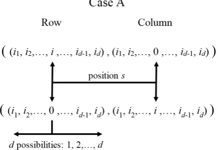
Case A is depicted in the Figure 1 for indexesI,Kbeing considered inDΨ_Id

4|Hli|ΨKd4 E

. There are a pair of entries whose labels for rows and columns have 0 or i in the position s = k: ((i1,i2, . . . ,i, . . . ,id),(i1,i2, . . . , 0, . . . ,id)) and ((i1,i2, . . . , 0, . . . ,id),(i1,i2, . . . ,i, . . . ,id)). This will be named the 0↔iassociation rule.

Figure 1. First case for a pair of entries in whichDΨId

4|Hli|ΨKd4

E

is non-zero. In them, for a fixed positions=kin the row and the column labels appearsior 0 alternatively, while other corresponding positions in the row and in the column have the same values.

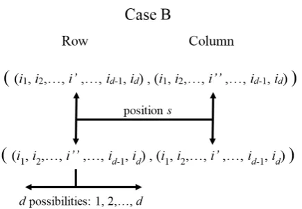
Case B is depicted in the Figure 2. Here, there are a pair of entries whose labels for rows and columns have i0 or i00 in the position s = k: ((i1,i2, . . . ,i0, . . . ,id),(i1,i2, . . . ,i00, . . . ,id)) and ((i1,i2, . . . ,i00, . . . ,id),(i1,i2, . . . ,i0, . . . ,id)), beingi,i0,i00a permutation of 1, 2, 3. This will be named the i0 ↔i00association rule.

At the end, clearly in each case, A or B, for each pair of correspondent interaction terms withiand kfix (k≤dandk+dpositions), there are only two pairs on non-zero entries in rows(i1,i2, . . . ,i, . . . ,id), (i1,i2, . . . , 0, . . . ,id)for the case A and in rows(i1,i2, . . . ,i0, . . . ,id),((i1,i2, . . . ,i00, . . . ,id))for the case B (with the corresponding column labels exchanged in both cases). They, together with diagonal entries generated by other adequate Hamiltonians (by exampleH0orHnl_i as it will be seen) will form

Figure 2.Second case for a pair of entries in whichDΨ_Id

4|Hli|ΨK4d

E

is non-zero. In them, for a fixed positions=kin the row and the column labels appearsi0ori00alternatively (beingi,i0,i00a permutation of 1, 2, 3), while other corresponding positions in the row and in the column have the same values.

h0,0...0,i,0,...,0withiin positionssord+s(meaning local interaction with each element of the pair of

correspondents parts in positionk). Noting that labels in the positions=kinI(row) andK(column) for the non-zero entries are 0,i;i, 0;i0,i00ori00,i0, then they cover all possibilitiesik=0, 1, 2, 3. Thus, for a fixed column and definedi,kvalues inDΨ_Id

4|Hli|ΨK4d E

, there is exactly one non-zero row; still, if two correspondentkelements are considered (local interactions on each element of a correspondent pair), they still generate only one non-zero row (each one with the two terms explained before).

Despite there are 2dpossibilities to select the positions=kin (25), they do not account as separate blocks because they appear in other entries in (21). Instead, for each term in non-correspondent terms, it will appear in a different non-zero row, givingdnon-zero rows as total; for eachidirection of interaction being included, additional non-zero rows will appear; last implies that 3d rows could appear when all parts have local interactions in the three spatial directions at time, destroying in this case the 2×2 block structure. Thus, maintaining local interactions in only one direction and on only one correspondent pair elements utmost, together, cases A and B form 1₂4d 2×2 blocks as it was required in the previous section. In any case, each non-zero entry will have the same 2 terms h_(i4k−1₎2d

4 with different signs depending onc is,ks

js,jd+s involved in each factor ofH (k)

li . Clearly, blocks can

be rearranged to order adequately the GBS basis elements getting the form (12). A brief analysis shows that there are not more diagonal-off elements in addition to last cases being generated by local terms. Additional diagonal-off elements are becoming from the non-local terms as those in Table 1.

4.3.3. Analysis ofDΨ_Id

4|Hnli|ΨKd4 E

With the correspondent parts definition and the analysis forHli, we can identify two cases for

the different termsH_nl(k,k0)

i : a) non-local interactions between correspondent parts, and b) non-local

interactions between non-correspondents parts. Discussion is similar to the previous subsection. Correspondent termsH_nl(k,k+d)

i . This term in the HamiltonianHnli containsσ0⊗...⊗σi⊗...⊗σi⊗...⊗ σ0withσiin positionskandk+d, andσ0in any other. When this term is allocated in

D

Ψ_Id

4|Hnli|ΨK4d E

in agreement with (21), it does not cancel if each factor in the product become different from zero, implyingis =ks ∀s=1, 2, ...,d. Thus, this term gives non-zero entries only in the diagonal elements. Thus, each non-zero entry ofHnli will haveddifferent terms in each diagonal element (one for each

pair of correspondent particles interacting). Those terms will appear with different signs in each diagonal element in spite ofcis,ks

js,jd+s. At this point, note that results forH (k,k+d)

nli andH

(k)

li were expected

Non-correspondent termsH_nl(k,k06=k+d)

i . These terms have a different behavior. Each term contains σ0⊗...⊗σi⊗...⊗σi⊗...⊗σ0 with σi in positionsk and k0, and σ0 in any other. It defines two

pairs of correspondent parts involving σi: [k,k+d,k0,k0+d]ifk < k0 ≤ d or k,k+d,k0−d,k0 if k≤d<k0 ≤2d. Then, each factor in (21) related with those two pairs (s=k,k0ors=k,k0−d) will include now Tr(σisσiσks)(until unitary factors), which is non-zero only if: a)isorksare one of the pairs

0 andioriand 0; b)i,is,ksare a permutationi,i0,i00of 1, 2, 3 (having two cases depending of the parity). Last situation is similar to the local terms in the previous subsection, but in two parts simultaneously. While, remaining factors fors6=k,k0ors6=k,k0−dwill requireis =ksin order to become non-zero. Last scenario gives 16 possibilities for each termh_(i(4k−1₊₄k0 −1₎₎2d

4 , which will appear in diagonal-off positions obtained departing from diagonal position(i1, ...,id;i1, ...,id)in

D

Ψ_Id

4|Hnli|ΨKd4 E

, by changing each one of indexes in the pair(ik,i_k0)in the row, following the rules depicted in the cases A and B. Thus, for each column andi,k,k0 fixed, only one row becomes non-zero in agreement with the previous rule. Each entry of this kind involves four terms including the four combinations of each two non-correspondent parts selected from the set[k,k0,k+d,k0+d]. Instead, when all valuesiandk,k0 are considered, a total of 3·1₂d(d−1)non-zero rows appear in each column (clearly, by considering all these terms,SU(2)decomposition is not achieved).

4.3.4. Analysis ofDΨ_Id

4|Hcnli|ΨKd4 E

Correspondent termsH_cnl(k,k+d)

i . For each termH (k,k+d)

cnl_i , the behavior is similar as forH (k0)

l_i . Due to only

one correspondent pair hasjp=js 6=06=jd+s=kpin (21), thenis,ksfors=k0should be 0,iorjp,kp. Fors6=k0,is =ks. As before, it means that each term is diagonal-off by combining the values of index k0inIandKas before: 0,i;i, 0;jp,kpandkp,jp. For a fixed column andi,kit will give four possibilities and twoSU(2)blocks. Each entry will have two terms corresponding to the different paritiesp. Note that only oneiandk0can be considered to achieve theSU(2)decomposition. Otherwise, for each column, could appear 3drows different from zero, breaking theSU(2)decomposition as for the local interaction case.

Non-correspondent termsH_cnl(k,k06=k+d)

i . As forH

(k,k06=k+d)

nli , in this case the only non-zero terms have

is = ks for s 6= k,k0,k−d,k0−d. While, for the two remaining cases s ∈ {k,k0,k−d,k0−d} ∩

{1, 2, . . . ,d}, eachis,ks should be selected from the set 0,jp; jp, 0; i,kp; kp,i or 0,kp; kp, 0; i,jp;jp,i. In a specific column and fixingi, it will give 16 possibilities and eight blocks inSU(2)as for the H_nl(k,k06=k+d)

i case. Note that parity p should be fixed in this case because each one give a different

decomposition. Each entry will contain four terms for each parity pcombining the four possible interaction terms. Again, if all options foriandk,k0,pare considered, then will appear 3·d(d−1) non-zero rows for each column, breaking theSU(2)decomposition. These kind of terms are non commonly introduced in models as Heisenberg-Ising and those related, instead for magnetic systems they are the first order approximation in the spin-orbit coupling introducing antisymmetric exchange as the Dzyaloshinskii-Moriya model:HDM =

− →

D·(−→σ1×−→σ2). There, − →

D is the Dzyaloshinskii-Moriya vector defining the orientation of coupling. Here, as only one term could be included in order to preserve theSU(2)reduction property, this coupling should be strictly oriented.

4.4. Explicit analytical formulas for Hamiltonians components

After last analysis, it is clear that other candidates to generateSU(2)decomposition are possible but they involve more than two parts at time (as theH0case), which are non-physical for common

point-like interactions, nevertheless these terms could appear for the quantum mechanical extended objects in which (1) is a merely expansion of the interactions. Therefore, we will restrict our remaining discussion to local or pairwise interactions. In this section, analytical formulas forDΨ_Id

4|Hli|ΨK4d E

, D

Ψ_Id

4|Hnli|ΨK4d E

andDΨ_Id

4|Hcnli|ΨKd4 E

their utility for computer simulation optimality purposes for larger systems. In order to simplify the expressions, we introduce the definition of the following generalized Kronecker delta:

δS_{I K}≡ d

∏

s∈/S

δ_isks (26)

where S is a set of scripts of excluded parts in the product. Thus, forHli:

D

Ψ_Id

4|Hli|ΨK4d E

= d

∑

δ{k

0_}

I K Hk

0

liId

4,Kd4

(27)

with : Hk0

l_iId

4,Kd4 =

1

∑

h_(i4k0+dt0 −1₎2d

4

Fiδ0,t0,iδ1,t0

i,k0

by notingcis,is

0,0 =1. InHk

0

liId

4,K4d

,[k0,k0+d]is the correspondent pair where each local interaction is being applied. There, the exchange factor generating the diagonal-off entries in theSU(2)blocks is:

F_ij_,,_kk0 = δi_k00δk_k0ic

0,i

j,k+δik0iδkk00c

i,0

j,k+

3

∑

e_ii20_i00δ_i

k0i0δkk0i00c

i0_,i00

j,k (28)

ForHnli:

D

ΨId

4|Hnli|ΨKd4 E

= d

∑

δ{k

0_}

I K Hc,k

0

nli Id

4,Kd4 +

d

∑

δ{k

0_,k00_}

I K Hnc,k

0_k00

nli Id

4,Kd4

(29)

with : Hc_nl,k0 iId

4,K4d

= h_(i(4k0 −1₊₄k0+d−1₎₎2d

4 δik0kk0c i_k0,i_k0

i,i

H_nlnc,k0k00 i Id

4,K4d =

1

∑

h_(i(4k0+dt0 −1₊₄k00+dt00 −1₎₎2d

4

Fiδ0,t0,iδ1,t0

i,k0 F

iδ_0,t00,iδ_1,t00

i,k00

each term belongs to correspondent and non-correspondent interactions respectively. InH_nlc,k0 i Id

4,Kd4 and

H_nlnc,k0k00 i Id

4,K4d

,[k0,k00]are the parts with non-local interactions between them. Similarly, forH_cnli:

D

Ψ_Id

4|Hcnli|ΨKd4 E

= d

∑

δ{k

0_}

I K H c,k0

cnliId

4,Kd4 +

1

∑

d

∑

δ{k

0_,k00_}

I K H

nc,k0k00p

cnli Id

4,K4d

(30)

with : Hc_cnl,k0 iId

4,Kd4 =

1

∑

h_(j

p4k0 −1+kp4k0+d−1)24dF jp,kp

i,k0

Hnc_cnl,k0k00p i Id

4,Kd4 =

1

∑

h_(j

p4k0+dt0 −1+kp4k00+dt00 −1)24dF

jpδ_0,t0,jpδ_1,t0

jp,k0 F

kpδ_0,t00,kpδ_1,t00

kp,k00

again,Hc_cnl,k0 iandH

nc,k0k00p

cnli are the correspondent and non-correspondent interactions in the Hamiltonian,

being[k0,k00]the parts where there are non-local interactions. It shows explicitly the existence of four (forHk0

li andH

c,k0

cnl_i) and sixteen (forH

nc,k0k00

nl_i andH

nc,k0k00p

cnl_i ) diagonal-off entries respectively in agreement

Note then, theSU(2)decomposition could be achieved only by: a) including any desired non-local termsHc_nl,k0

i (to generate the diagonal elements); and b) including only one type of interaction among Hk0

li,H

nc,k0k00

nli ,H

c,k0

cnli orH

nc,k0k00p

cnli for concrete values fori,k

0_,k00_andp. An important property used later forFjs,jd+s

i,k0 is that only one term utmost in (28) remains with the election ofik0andk_k0. Due to eachc_jj_,s_k,jd+s is real or imaginary, and more concretely, as a brief analysis

shows that if it is not zero, then it becomes imaginary only ifjsor jd+sis equal to 2, therefore this property is transferred toFjs,jd+s

i,k0 .

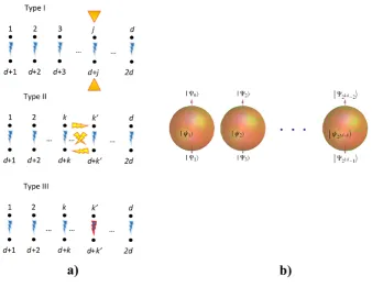
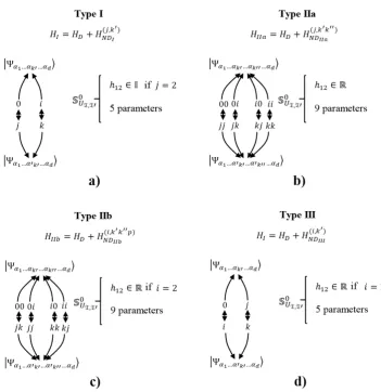
5. Specific interactions generatingSU(2)decomposition

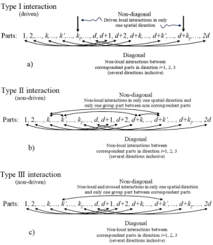
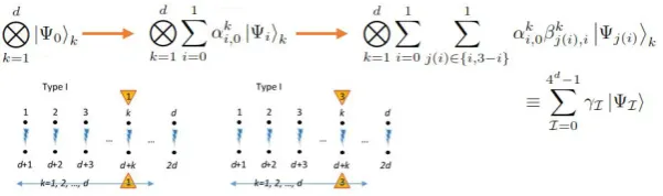
In this section, we summarize and organize the global findings to reach theSU(2)block structure on the GBS basis. Finally, we will conclude that there are three great types of interactions able to generate the block structure as it was depicted in section 3.

5.1. General depiction of interactions having SU(2)decomposition for the GBS basis

Based on the previous discussion, there are three groups of interactions able to generate the SU(2)decomposition on the GBS basis. The first one (Type I) comprehend all kind of non-local and non-crossed interactions between any two correspondent parts in any direction. These terms generate the diagonal terms depicted before in the Hamiltonian. Together, only two local interactions in only one specific direction and on only one pair of correspondent parts,kl, should be included to generate the diagonal-off entries. Thus, this group of interactions conform theSU(2)blocks. Note that local interaction terms could be intended as external driven fields as in [8,23]. The second interaction (Type II) is obtained by substituting the previous local interactions with non-local interactions among only those non-correspondent elements included in two pairs of correspondent parts. It means, if k,k0,k+d,k0+dwithk< k0 ≤ dare these elements in the two correspondent parts, then only the interactions between the following non-correspondent elements are allowed:[k,k0],[k,k0+d],[k0,k+d] and[k+d,k0+d]. This group of four interactions generates the diagonal-off terms to conform the SU(2)blocks. Nevertheless, Type II interaction normally should be understood as a non driven process of control. Note that Type II interaction could be classified in two other subclasses: a) Type IIa for non-crossed interactionsHnc_nl,k0k00

i , and b) Type IIb for crossed interactionsH

nc,k0k00p

cnli . Finally, the

third interaction (Type III) comprehend together: the non-local and non-crossed interactions with the inclusion of crossed interactions between one specific correspondent pair.

Figure 3 resumes the three types of interactions depicted before. In particular, note this description is in agreement with the results in the Table 1 ford=1, despite it is an special case because diagonal-off entries for Type I, II and III coincide in the same diagonal-off entries, so both interactions could be combined at same time preserving theSU(2)decomposition. This case has a richer structure for control in terms of the number of free parameters involved with respect to the number of parts to be controlled. Note that while Type I and III only are able to modify the inner entanglement of the correspondent pairs, Type II interaction lets to generate of modify the global entanglement between different correspondent pairs, thus letting spread it on the entire system by switching the pairs involving interactions generating diagonal-off entries.

5.2. General structure of SU(2)blocks

In this subsection a complementary analysis ofSU(2)blocks obtained for the last interactions will be given. Their form is particularly useful as a connection with optimal control schemes as those presented in [6]. In any case (Type I, II or III), each blockSHI,I0 (withI,I0 the rows in which is

Figure 3.Three types of physical interactions able to generate the block decomposition. Non-local and non-crossed interactions among any correspondent parts combined with: a) local interactions on only two correspondent parts (kl,kl+d), b) any two non-correspondent parts in only two specific pairs of correspondent parts of only one subtype, non-crossed or crossed, and c) crossed interactions between a specific pair of correspondent parts.

SHI,I0 = h11 h12

h∗₁₂ h22

!

(31)

= h11+h22

2 II,I0+Re(h12)XI,I0−Im(h12)YI,I0+

h11−h22

2 ZI,I0

where{II,I0,_XI,I0,_YI,I0,_ZI,I0}is the Pauli basis for theSU(2)block. If the Hamiltonian coefficients

involved in the block are time independent, then the correspondingSUI,I0 block in the evolution

SUI,I0 = eiSHI,I 0ht¯ _=ei

h₁₁+h₂₂

2¯h teiωn·sI,I 0t_=eih11

+h₂₂

2¯h t(cos_ωt+isin_ωtn·s_I,I0) (32)

= eih11 +h₂₂

2¯h t cosωt+i

h11−h22

2¯hω sinωt i

h12

¯

hω sinωt ih∗12

¯

hωsinωt cosωt−i h11−h22

2¯hω sinωt

!

with : n= 1 ¯

hω(Re(h12),−Im(h12),

h11−h22

2 )

sI,I0 = (_XI,I0,_YI,I0,_ZI,I0)

¯ hω=

r

|h12|2+

1

4|h11−h22|

2

clearly belonging toU(1)×SU(2). As was stated before,Fjs,jd+s

j,k0 is imaginary only ifjs orjd+sis 2. Thus, only one component fromn1orn2is different from zero because non-diagonal entries of block

in (27,29,30) are always real or imaginary. It reduces the optimal control to the second case reported by [6]. An additional analysis will show thath11±h22 6=0 in general (without impose restrictions to the

non-local strengthshJ), this aspect will be relevant after.

5.3. Structure of SU(2)blocks for each interaction

Several classical interactions fitting in the current procedure have been analyzed. All them generate blocks (no necessarilySU(2)blocks) when they are expressed in the GBS basis, denoting a kind of universality for this basis due to its ability to gather up similar interactions through simplified representations. In the sake of the search ofSU(2)decomposition, we discuss finally closed forms for the specific Hamiltonians able to achieve theSU(2)decomposition.

5.3.1. Blocks in Type I interaction

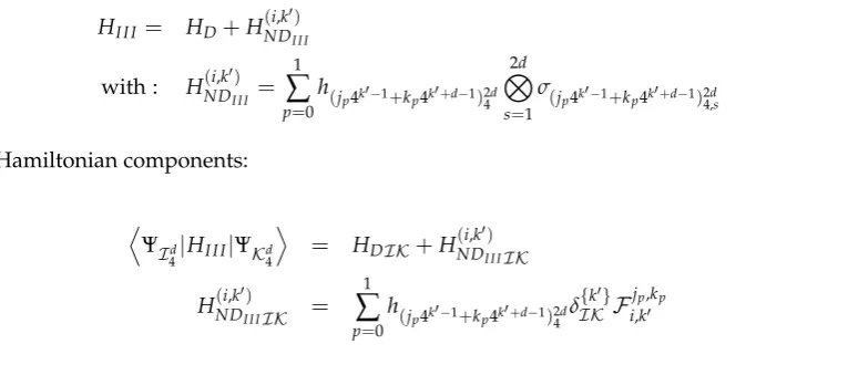
This interaction includes non-crossed spin interactions between correspondent particles in all spatial directions and external local interactions on the pair[k0,k0+d]of correspondent particles in directionj. From (27-29), it can be written as:

HI = HD+H(j,k

0₎

NDI (33)

with : HD ≡

3

∑

d

∑

h_(i0₍₄k−1₊₄k+d−1₎₎2d

4

2d O s=1

σ_(i0₍₄k−1₊₄k+d−1₎₎2d

4,s

H(_NDj,k0_I)=

1

∑

h_(j4k0+dt0 −1₎2d

4

2d O s=1

σ_(j4k0+dt0 −1₎2d

4,s

generatingSU(2)blocks with the diagonal terms from non-local interactions between correspondent parts and the non-diagonal terms from local interactions. Departing from (27-29), we get for the Hamiltonian components:

D

ΨId

4|HI|ΨK4d E

= δI K

3

∑

d

∑

(−1)δi0,2+(1−δi0,i_k00)(1−δ0,i_k00)_h

(i0₍₄k00 −1₊₄k00+d−1₎₎2d

4

+

1

∑

h_(j4k0+dt0 −1₎2d

4 δ

{k0} I K F

jδ_0,t0,jδ_1,t0

j,k0 ≡HDI K+H(j,k

0₎

NDII K (34)

last formula is obtained noting thatcik00,ik00

i,i = (−1)

δi,2+(1−δi,i_k00)(1−δ0,i_k00)_{. The first term of last expressions}

the diagonal of eachSU(2)block are different. Due to the block is formed by switching an indexik00

in the rows labels (or two as in the following cases) in agreement with the association 0↔jori↔k (jis the direction associated to the interaction andi,j,ka permutation of 1, 2, 3), then fori0 6= jthe terms inHDI Khave a sign change. It implies that in generalh116=h22in (31), generating non-diagonal

SHI,I0-blocks. The second term contains the four diagonal-off elements generating two blocks with

two terms each one. Note that Hamiltonian terms (hI) are real together withc i_k00,i_k00

i,i , so diagonal terms are real as is expected. Diagonal-off terms will be real or imaginary depending fromF_jj_,,0_k0,F

0,j

j,k0. In any

case, concretely, they are imaginary only ifj=2.

Clearly, note that this interaction applied on a combination of correspondent pairs with bipartite entangled states generate only non-local operations on each correspondent pair as those presented in [8,10]. Still switching the directionjand the correspondent pairk0on which the local interaction is applied, this kind of Hamiltonian cannot generate extended entanglement between correspondent pairs more than the included in the initial state. It means that if the initial state is separable by correspondent pairs, it will remain separable at this level (but should be able to entangle or untangle the parts of each pair). Conversely, it cannot untangling each correspondent pair from the remaining state in more complex cases. We deserve a later section to analyze these topics.

5.3.2. Blocks in Type II interaction

Type IIa :In this case, interaction is completely non-local between correspondent pairs to generate the diagonal entries and in only one direction between non-correspondent parts in two correspondent pairs to generate the diagonal-off entries. Hamiltonian becomes:

HI Ia= HD+H(j,k

0_k00₎

NDI Ia (35)

with : H(_NDj,k0k00)

I Ia = 1

∑

h_(j(4k0+dt0 −1₊₄k00+dt00 −1₎₎2d

4

2d O s=1

σ_(j(4k0+dt0 −1₊₄k00+dt00 −1₎₎2d

4,s

with a non-local and non-crossed interaction in the directionjfor the group of non-correspondent terms defined byk0<k00≤d. The Hamiltonian entries are similar to those in (27-29) but with the last restriction for the non-correspondent terms of interaction. Due to discussion in the previous subsection, diagonal-off entries in the Hamiltonian are now always real. Components become:

D

ΨId

4|HI Ia|ΨKd4 E

= HDI K+H(j,k

0_k00₎

NDI Ia I K (36)

H(_NDj,k0k00)

I Ia I K ≡

1

∑

h_(j(4k0+dt0 −1₊₄k00+dt00 −1₎₎2d

4 δ

{k0,k00} I K F

jδ_0,t0,jδ_1,t0

j,k0 F

jδ_0,t00,jδ_1,t00

j,k00

Type IIb :For this interaction, the non-diagonal part generated by the non-local interaction between non-correspondent parts is supplied by a non-local and crossed interaction among non-correspondent parts of two pairs of correspondent pairs:

HI Ib= HD+H(i,k

0_k00_p)

NDI Ib (37)

with : H(_NDi,k0k00p)

I Ib ≡ 1

∑

h_(j

p4k0+dt0 −1+kp4k00+dt00 −1)2₄d 2d O s=1

σ_(j

p4k0+dt0 −1+kp4k00+dt00 −1)2_4,d_s

D

ΨId

4|HI Ib|ΨKd4 E

= HDI K+H(i,k

0_k00_p)

NDI Ib I K (38)

H(_NDi,k0k00p)

I Ib I K =

1

∑

h_(j

p4k0+dt0 −1+kp4k00+dt00 −1)2₄dδ {k0,k00} I K F

jpδ_0,t0,jpδ_1,t0

jp,k0 F

kpδ_0,t00,kpδ_1,t00

kp,k00

the non-diagonal entries are now imaginary, except fori=2. 5.3.3. Blocks in Type III interaction

Finally, for Type III interaction, the non-diagonal part is generated by the non-local and crossed interaction between a pair of correspondent partsk0:

HI I I = HD+H(i,k

0₎

NDI I I (39)

with : H(_NDi,k0)

I I I = 1

∑

h_(j

p4k0 −1+kp4k0+d−1)24d

2d O s=1

σ_(j

p4k0 −1+kp4k0+d−1)24,ds

with the Hamiltonian components:

D

ΨId

4|HI I I|ΨKd4 E

= HDI K+H(i,k

0₎

NDI I II K (40)

H(_NDi,k0)

I I II K =

1

∑

h_(j

p4k0 −1+kp4k0+d−1)2₄dδ {k0} I K F

jp,kp

i,k0

where non-diagonal entries are imaginary only ifi=2.

Figure 4 depicts the three types of interactions associated with theSU(2)decomposition. Rays represent non-local interactions (blue/dark between correspondent particles and yellow/bright between non-correspondent ones), while the yellow wedges mark particles subject to external local driving interactions. Distributed evolution on 22d−1 Bloch spheres is shown for the states

ψ_j

=α2j−2

Ψ_2j−2+α2j−1

Ψ_2j−1which are part of the global state|ψi=∑22d

−1 j=1

ψ_j

, where each

|Ψkiis an element of the GBS basis. Each state ψ_j

evolves as a different curve on each Bloch sphere depending on parametershJ.

Finally, we should note that each one of the last interactions involves labels to be completely identified, namely:H_I(j,k0),H_{I Ia}(j,k0,k00),H_{I Ib}(j,k0,k00,p)andH_{I I I}(j,k0,k00). These labels will be omitted by simplicity at least their specification becomes needed. In any case, closed expressions (34, 36, 38, 40) are computationally efficient to generate matrix representations of HamiltoniansHI,HI Ia,b,HI I I, then for

their respectiveU, inclusively in the time dependent case, despite a numerical approach to construct could be necessary.

5.4. Available parameters and structure of entries

Figure 4.Representation of qubit interactions able to generateSU(2)decomposition: a) Type I, II and III interactions among 2dqubits (Type III assumes the inclusion of crossed interactions in the pairk0), and b) Distributed evolution on 22d−1_{Bloch spheres, each one for the states}

ψj E

.

the exponential grow of the matrix with the system sized) to set a whole control (over all blocks) in one period of constant driven parameters, suggesting the use of time dependent or at least a constant-piecewise parameters to increase the control.

Table 2.Rows generated and free parameters in each interaction considered in the text.

Hamiltonian Entries type Entries by column/row Parameters by entry

H0 Diagonal 1 D≤3

Hli Non-diagonal d 2

H_nlic Diagonal 1 d

H_nlinc Non-diagonal 1₂d(d−1) 4

Hc

cnli Non-diagonal d 2

Hnc

cnli Non-diagonal d(d−1) 4

HI 2×2 block 2 2+Dd≤2+3d

HI Ia,b 2×2 block 2 4+Dd≤4+3d HI I I 2×2 block 2 2+Dd≤2+3d

5.4.1. Structure of diagonal entries belonging to a specific block

Other aspects should be remarked. The first one is related with terms in the diagonal entries generated by non-local interactionsHc_nl,s

jamong correspondent parts. Note that blocks are generated by

other interactions to those, which are prescribed as a difference in one (H_nlc,k0 i orH

c,k0

cnli) or two (H

nc,k0k00

nli

orHnc_cnl,k0k00p

i ) terms in the scripts labels in agreement with the rules depicted in the Figures 1 and 2. It

implies there will be two or eight blocks each one relating rows (and columns) differing in only one or two terms of their scripts respectively. We can note for the diagonal entries forHc_nl,s

jin (21) for the

fix correspondent pair, there will be only four signs combinations (none is the negative of another) depending on: a) the direction of the interaction involved (on the correspondent pairs) isj =2 or j6=2, and b)isfor thesthscript is in the set{0,j}or in{i,k}(withi,j,ka permutation of 1, 2, 3). There, the factors corresponding to other correspondent pairs will be equal to one. Then, for the 3dterms included in all diagonal entries will be 4dcombinations for the whole terms, precisely the number of rows! It implies that all diagonal entries are different (but not linearly independent because there are only 3dparameters). Despite, for two rows differing in only one or two terms in their scripts, only the three or six terms corresponding with the strengths ofHc_nl,s

j for such correspondent pairs (associated

with those terms in the scripts) will change their signs in the diagonal terms in their block. As a consequence, for such 4d−1or 4d−2groups of blocks having the same scripts exchange and generated by the whole combinations in the otherd−1 ord−2 terms in their scripts, they will have the same h11−h22parameters respectively. Thus, it will be only two or eight differenth11−h22parameters for

the entireH. While,h11+h22parameters could be different.

5.4.2. Structure of diagonal-off entries belonging to a specific block

The second aspect is related with the explicit calculation ofcis,ks

js,jd+s for the basic interest cases in

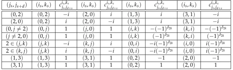
the diagonal-off entries. a) ForHIandHI Ia,b:js =j,jd+s =0 orjs=0,jd+s =j(beingjthe direction label involved in the local and non-local interactions between non-correspondent parts; b) and b) for HI I I:js =jp,jd+s =kp. Table 3 shows explicitly these values. Note the parallelism between the two halves of them (vertically and horizontally).

These cases generate the diagonal-off entries in each block in agreement with the exchange rules depicted before for thesth_{scripts of such entries’ rows:(i}

s,ks)∈ {(0,j),(j, 0);(i,k),(k,i)}, withi,j,ka permutation from 1, 2, 3 andjthe associated direction for the corresponding interaction being used fromHIandHI Ia,b; and,(is,ks)∈ {(jp,kp),(kp,jp);(0,i),(i, 0)}, withi,jp,kpa permutation of parityp

from 1, 2, 3 andjp,kpare the associated directions for the interactionHI I I.

We should note first that signs for each term in the diagonal-off entries do not depend on the entries’ scripts in the other positions than the parts in which interaction is being applied,k0,k00in the expressions of the previous section (33,35,37,39). It is because Tr(σ˜_i∗

sσjd+sσ˜

T ksσ

T

js) =Tr(σ˜ ∗ isσ0σ˜

T ksσ

T

0) =2 .

Instead, signs only depend on the type of exchange indexes shown in the Table 3. Other fact already noted is thatcis,ks

js,jd+s is imaginary only ifjs = 2 orjd+s = 2. This property is then transferred to the

correspondingFjs,jd+s

j,s and then transformed toh12 as a function of the number of those factors in

(34,36,38,40). Thus, by exchangingis,ks(block transposing), only the cases withh12 ∈Iwill change

their sign.

The final fact is related with the different signs appearing in the terms of diagonal-off entries. This aspect will be important to analyze the number of independent blocks in the entire evolution matrix. ForHIandHI I Ithe two different terms are obtained by the exchange ofjs,jd+s. Thus, forHI, only the

cis,ks

js,jd+s with(js,js+d) = (0, 2),(2, 0)and(is,ks)∈ {(0, 2),(2, 0)}or(js,js+d) = (0,j6=2),(j6=2, 0)and

(is,ks)∈ {(i,k),(k,i)}will change their sign (in the first four rows of Table 3). ForHI I I, if(js,js+d) = (1, 3),(3, 1)and(is,ks) ∈ {(0, 2),(2, 0)}or(js,js+d) = (0, 2),(2, 0)and(is,ks) ∈ {(i,k),(k,i)}, then cis,ks

js,jd+s will change their sign (in the last four rows of Table 3). ForHI Ia,b, two terms in the scripts are

involved, so different aspects contribute: location of parts interacting, type of exchange and their order in the scripts.

This aspect exhibits the way in which each term inh12will change or will not their sign. These

due to the entries ofSUdepend only on the parametersh11±h22,h12. As a result, as we will seen, by

grouping finally in theU(1)×SU(2)blocks, there will only two or eight different blocksSUinU.

Table 3.Values ofcis,ks

js,jd+sfor all exchange scripts inHI,HI Ia,b,HI I I.i,j,kis an even permutation of 1, 2, 3 (js,js+d) (is,ks) c_jis,_s,k_jd+ss (is,ks) ci_js,_s,k_jd+ss (is,ks) c_ji_s,s,k_jd+ss (is,ks) ci_js,_s,k_jd+ss

(0, 2) (0, 2) −i (2, 0) i (1, 3) i (3, 1) −i (2, 0) (0, 2) i (2, 0) −i (1, 3) i (3, 1) −i (0,j6=2) (0,j) 1 (j, 0) 1 (i,k) −(−1)δ2k _{(k,i) −(−1)}δ2k (j6=2, 0) (0,j) 1 (j, 0) 1 (i,k) (−1)δ2k _{(k,i) (−1)}δ2k

2∈(j,k) (j,k) −i (k,j) i (0,i) −i(−1)δ2k _{(i, 0) i(−1)}δ2k

2∈(k,j) (j,k) i (k,j) −i (0,i) −i(−1)δ2k _{(i, 0) i(−1)}δ2k (1, 3) (1, 3) 1 (3, 1) 1 (0, 2) −1 (2, 0) −1

(3, 1) (1, 3) 1 (3, 1) 1 (0, 2) 1 (2, 0) 1

5.4.3. Block entries ofHI

The diagonal-off entries have exactly the two termsh_(j4s+dt−1₎2d

4 fort

0 _{=0, 1 and there are only} two combinations: adding or subtracting terms. As was stated previously, they are imaginary only if local interactions are in directionj=2. If in such case we separate the factor±iforj=2 cases in the diagonal-off entries, the remaining coefficients in the opposite corners in each block are equal as is expected in (31). Then, in general, there is one term with the same sign through all diagonal-off entries (depending ifk=2 or not, or otherwise ifjs =2 in the first four rows in the Table 3), leaving only two possibilities for the remaining term. Thus, in eachHImatrix there are blocks with only two different diagonal-off entries, only depending on the indexes exchange type in the local interaction position but not on the remaining indexes. Thus, for a fixed set of indexes for the positions do not related with the part on which the interaction is applied, a pair of blocks exists, each one for the exchanges(0,j),(j, 0) and(i,k),(k,i), with different relative signs in their diagonal-off terms. For the corresponding diagonal entries, in (32), only the differenceh11−h22is relevant. As was previously stated by analyzing the

formula (34), it is also possible realize that in each diagonal entry there are only two terms from the 3dterms changing their sign with respect to other rows. Block scripts differ in only one index, those corresponding withi0 6=j(the local interaction direction) andk=k0(the correspondent pair on which local interaction is being applied), leaving only two terms and two different combinations forh11−h22.

It implies there are only two different blocks for (32) through allU, operating each one with different exchange rules,(0,j),(j, 0)or(i,k),(k,i). Each one is the same (until unitary factors which could be different) for all entries with different indexes in other positions thank0. This fact appoints, depending on the disposable number of parameters (five, including the time and excluding the parameters in the unitary factor of each block), to the independence between the two types of blocks in the evolution matrix (32).

5.4.4. Block entries ofHI Ia

In this case, for the non-diagonal entries, due to the exchange factorFjs,jd+s