1
Some new light on the study of fluid flow in closed conduits:
1
An experimental protocol to identify the value of a misconstrued constant
2 3
Hubert M Quinn; 4
The Wrangler Group LLC, 40 Nottinghill Road, Brighton, Ma.02135; [email protected]: 857-540-0570:
5 6 7
Abstract 8
9
In this paper, the experimental protocol which we disclose is designed to identify the values for 10
both the constant in the Kozeny/Carman model, which relates to the linear component of 11
permeability, and the variable kinetic coefficient in the newly minted Q- modified Ergun model, 12
which relates to the non-linear components of permeability, without involving any new 13
theoretical development. Moreover, kinetic contributions to measured pressure gradient, 14
which are not accounted for in some currently accepted empirical fluid flow equations, such as 15
Poiseuille’s for flow in empty conduits and Kozeny/Carman for flow in packed conduits, but 16
which nevertheless contribute to measured pressure drop and thus hamper the identification 17
of the value of the constant relative to the laminar component, are captured and lumped 18
together into a single variable kinetic parameter-the kinetic coefficient. 19
20
Keywords: Bed Permeability: Kozeny/Carman: Ergun: Friction Factor: Porosity: UHPLC. 21
44
1. Introduction 45
46
Beginning with the work of Darcy in packed conduits circa 1856 and continuing to this very day, 47
extraordinary amounts of energy has been expended by authors of scientific publications in an 48
attempt to shed light on an understanding of underlying contributions to permeability, not only 49
in packed conduits, but also in empty conduits [1]. 50
51
Azevedo et al focused their attention on turbulent flow of water in corrugated pipes [2]. Baker 52
et al studied the flow of air through packed conduits containing spherical particles [3]. Erdim et 53
al studied the pressure drop-flow rate correlation of spherical powdered metal particles in 54
packed conduits [4]. Dukhan et al, studied pressure drop in porous media with an eye to 55
reconciliation with classical empirical equations [5]. Anspach et al reported results relating to 56
very high pressure drops in very narrow id HPLC columns using small fully porous particles [6]. 57
Zhong et al. studied air flow through sintered metal particles in the context of the Ergun flow 58
model [7]. Tian et al reported experimental results with sintered ore particles in packed 59
conduits [8]. Mayerhofer et al studied the permeability of irregularly shaped wood particles [9]. 60
Pesic et al studied the effect of temperature on permeability of packed conduits containing 61
spherical particles [10]. Abidzaid et al discusses water flow through packed beds in light of 62
some modified equations [11]. Mirmanto et al studied friction factor of water in micro channels 63
[12]. Capinlioglu et al focused his work on simplified correlations of packed bed pressure drops 64
[13]. Yang et al made comparisons of superficially porous particles in packed HPLC columns 65
[14]. Lundstrom et al used sophisticated analysis techniques to evaluate transitional and 66
turbulent flow in packed beds [15]. Sletfjerding et al reported on flow experiments with high 67
pressure natural gas in empty pipes [16]. Langeiandsvik et al studied pipeline permeability and 68
capacity [17]. De Stephano et al studied the performance characteristics of small particles in 69
packed conduits for fast HPLC analysis [18]. Pereira reported on expected pressure drops in 70
commercial HPLC columns [19]. Van Lopik et al studied grain size on nonlinear flow behavior 71
[20]. Li et al discussed particle diameter effects in sand columns [21]. An in depth evaluation of 72
each one of the references above can be found on our web site;www.wranglergroup.com/UPPR 73
74
In our appreciation for the historical record regarding the work of renowned contributors in the 75
field of permeability as applied to flow in closed conduits, we have given equal consideration to 76
all classical works in both packed and empty conduits. Because the field of general engineering 77
in empty conduits is so vast, it is beyond the scope of this paper. Nevertheless, it is part of the 78
same fundamental science and any serious fluid dynamic assessment must include it in its 79
repertoire, especially when challenging conventional wisdom, as we are doing here. 80
Accordingly, as part of our foundation in challenging conventional wisdom with regard to 81
permeability in packed conduits, and particularly in chromatographic columns, and even more 82
particularly, in the recent vintage so-called sub 2 micron high throughput analytical columns, 83
recent work which we will refer to here as the Princeton study (circa 1995) [24]. Since these 87
classical works in empty conduits are directly supportive of our thesis herein concerning 88
permeability in packed conduits, we include as part of our assessments herein the teaching of 89
Poiseuille’s which is broadly accepted as the governing equation underlying permeability in 90
empty conduits in the laminar flow regime, which is a specific target of this paper. 91
92
We would be remiss herein however, if we did not single out for special mention the works of 93
two popular authors whose work in packed chromatographic columns we consider legendary. 94
Those authors are Sabri Ergun [25,26] and Georges Guiochon [27]. 95
96
Firstly, we believe that, with respect to the values of his equation “constants”, Ergun got it 97
completely wrong for a variety of reasons which we go into in great detail in another 98
publication [28]. Suffice it to say in this writing that, although we acknowledge that Ergun made 99
a unique, significant and lasting contribution to the underpinnings of fluid dynamics, by virtue 100
of his putting together two distinct elements of viscous and kinetic expressions for energy 101
dissipation in packed conduits, his work has been memorialized by many for the wrong reasons-102
his erroneous assignment of the now famous values of 150 and 1.75 for the “constants” of his 103
now equally famous Ergun equation. 104
105
Guiochon, on the other hand, although he published a prestigious amount of experimental 106
data, is famous for taking one step forward and two steps backward in his continuous flip-flop 107
assertions concerning the value of the constant in the Kozeny/Carman equation [29]. His work 108
will be remembered for his contention that the value of the constant could be anything from 109
120 to 300 and, despite the fact that, occasionally, he would assign a very specific value 110
depending on the results of a particular experiment in hand, he would often times, either revert 111
backwards to the safety of Darcyism or further seek shelter in the vague proclamation that the 112
value of the constant was a complete mishmash of undetermined variables [30]. 113
114
In order to facilitate a comprehensive understanding of fluid flow in closed conduits, therefore, 115
one must develop a common language which crosses the chasm between empty and packed 116
conduits, on the one hand, and laminar and turbulent flow regimes, on the other. Let us begin 117
with the language of a typical chromatographer who invariably invokes the permeability 118
parameter K0, a dimensionless mathematical construct.
119 120
Conduit permeability may be expressed, as follows; 121
122
P = s (1)
123
L 124
125
Where, P is the pressure differential between the inlet and outlet of the conduit; L is the 126
length of the conduit;s is the superficial fluid velocity; is the fluid absolute viscosity and K0,
is conduit permeability based upon the use of superficial fluid flow velocity, s, and where
128
superficial velocity,s, in turn, is defined as:
129 130
s = q (2)
131
D
132 133
Where, D = conduit diameter and q = fluid volumetric flow rate.
134 135
Let us define the term “friction factor”, f, which is widely used jargon relating to flow in 136
conduits, as a dimensionless mathematical construct which normalizes pressure drop in a 137
conduit for the various individual contributions to that pressure drop value and is the reciprocal 138
of K0. In the case of an empty conduit and when the flow regime is confined to that of laminar
139
flow, it is defined as; 140
141
fP =P (3)
142
sL
143 144
= (4)
145
K0
146 147
Where, fp is the Poiseuille’s type friction factor.
148 149
1.1The Poiseuille’s and Kozeny/Carman Models 150
151
Readers familiar with fluid dynamics will recognize that when it comes to laminar flow, 152
Poiseuille’s equation is generally considered the governing permeability equation in an empty 153
conduit and the Kozeny/Carman equation is generally considered the governing permeability 154
equation in a packed conduit. Let us further examine these two relationships. 155
156
Poiseuille’s equation can be written as; 157
158
P = 32s (5)
159
L D2 160
161
Rearranging gives: 162
163
PD2 = 32 (6)
164
sL
166
Substituting K0 in equation (1)into equation (6) gives:
167 168
D2 = 32 (7)
169
K0
170 171
= KP (8)
172 173
Where, Kp,is defined as Poiseuille’s constant for laminar flow.
174
175
Similarly, the Kozeny/Carman equation can be written as: 176
177
P = Kcvs (9)
178
L dp2
179
180
Where, KC= Kozeny/Carman constant, dp = the average spherical particle diameter equivalent
181
and v = the viscous porosity dependenceterm.
182 183
And where, the porosity dependence term, v , in turn, is refined as:
184 185
v = (
186
o3
187 188
Where,o= the external porosity of the packed conduit, also defined as;
189 190
o = Ve
191
Vec
192 193
Where, Ve = the volume external to the particle fraction and Vec = the empty volume of the
194
conduit in the packed column. 195
196
We point out here that variations in specific surface area are accommodated within our 197
concept of spherical particle diameter equivalent, i.e., the value of dp.
198 199
Similarly, as in the case of the Poiseuille model, the Kozeny/Carman model maybe expressed as 200
a dimensionless friction factor. This is accomplished by normalizing the pressure drop term in 201
equation (9), on the left hand side of the equality sign, for the individual contribution terms, on 202
204
Pdp2 = fK (12)
205
vsL
206 207
Where, fK is the Kozeny/Carman type friction factor.
208
209
Isolating the term Kc, as a dimensionless mathematical construct, by rearranging equating (9)
210
gives: 211
212
Kc = Pdp2 (13)
213
vsL
214 215
Substituting K0 into equation (13) gives:
216 217
Kc = dp2 (14)
218
K0v
219 220
Note that there is an embedded numerical coefficient, 32, in the Poiseuille model which we 221
have written as equation (7) and in equation (8) assigned the symbol KP and the label
222
Poiseuille’s constant. However, in equation (13) for the Kozeny/Carman model, although we 223
have the term KC which we label the Kozeny/Carman constant, there is no numerical value
224
assigned to it. Since both equations purport to represent permeability in a closed conduit when 225
the fluid flow is laminar, let us assume that they both represent the same functional concept in 226
each equation and that they are, therefore, related. 227
228
Accordingly, let us functionally equate the formulae embedded in the Poiseuille model and in 229
the Kozeny/Carman model as follows: 230
231
Kc = dp2 (15)
232
KP D2v
233 234
Substituting for KP into equation (15)and rearranginggives;
235 236
Kc = dp2 (16)
237
D2v
238 239
Where, functional equivalency between the two fluid flow models is dictated by two internally 240
242
The term dp in the Kozeny/Carman model = the term D in the Poiseuille model, and
243
the term v in the Kozeny/Carman modelhas the constant numerical value of 0.125 (1/8) in the
244
Poiseuille model. 245
246
We can now derive a more specific version of both the Poiseuille and the Kozeny/Carman 247
models by, on the one hand, importing the concept of porosity from the Kozeny/Carman model 248
into the Poiseuille model, and, on the other hand, importing the numerical value of the 249
constant from the Poiseuille model into the Kozeny/Carman model. Thus, we can represent our 250
equalizing and reciprocating boundary conditions as: 251
252
dp= D; v8 (17)
253 254
Incorporating this assumption into equation (16) gives: 255
256
Kc = KP = 32 = (18)
257
v (1/8)
258 259
Equation (18) would appear to suggest, however, what appears to be a contradiction in terms, 260
i.e. the value of the constant in the Poiseuille model, KP, has two confliction values, i.e. 32 and
261
256. To demonstrate that these two numerical values do not represent a contradictory 262
interpretation of the Poiseuille model, let us further articulate the meaning of what our 263
equivalency proposition actually represents. We do this by recasting the Poiseuille model in 264
both of its now dual dimensionless friction factor formats. To accomplish this, we initially 265
express the Poiseuille model in terms of the Poiseuille type friction factor as follows: 266
267
fP = PD2 = 32 (19)
268
sL
269 270
Note that in this format, the characteristic dimension of the conduit is expressed in terms of its 271
diameter D. 272
273
Similarly, we may now express the Poiseuille model in terms of a Kozeny/Carman type friction 274
factor by incorporating our equalization assumptions, as follows: 275
276
fP = PD2 = 256 (20)
277
vsL
How can we justify that equations (19) and (20) are two equivalent renditions of the same 280
entity? The answer lies in the Conservation Laws of Nature sometimes referred to as the Laws 281
of Continuity when they involve moving entities. In any conduit packed with particles, the total 282
free space contained within the conduit is proportioned between the volume fraction taken up 283
by the particles and the volume fraction taken up by the fluid. Accordingly, the characteristic 284
dimension of the particles contained in a conduit and the resultant conduit porosity are not 285
independent variables, meaning the one depends upon the value of the other. 286
287
In the case of a conduit packed with particles, since the particle diameter, dp, may vary
288
independently of the conduit diameter, D, the ratio of the conduit diameter to the particle 289
diameter, D/dp, may vary over a very wide range of values, and accordingly, the value of the
290
packed column external porosity, 0, also may vary over a very broad range of values. The first
291
functional boundary conditions which we imposed upon the Poiseuille model - which applies 292
only to an empty conduit- simply demonstrates that resultant porosity, in the case of an empty 293
conduit, is always a constant because we defined the ratio of conduit diameter to particle 294
diameter to be a constant, i.e. D/dp = 1 (unity). Therefore, the permeability of an empty conduit
295
is represented in terms of (a) its diameter in conjunction with a numerical coefficient in which 296
the constant value of its porosity is embedded where KP = 32 or (b) its diameter in conjunction
297
with a numerical coefficient which does not contain the constant value of porosity embedded 298
but, instead, the constant value of the porosity is expressed in the separate term v where KP =
299
256. In the case where the conduit porosity is expressed in the separate termv whose value =
300
1/8, the value of 256 is greater because the external porosity, in an empty conduit is not 301
only constant but it is also greater than unity. In fact, the value of the porosity dependence 302
term v in an empty conduit (1/8) is the correlation coefficient between these two numerical
303
values representing the constant in the respective dimensionless formats for an empty conduit. 304
305
1.2The Ergun Model 306
307
Having established a frame of reference for hydrodynamics between an empty and a packed 308
conduit in the regime of laminar flow, where permeability is a linear function of fluid flow 309
velocity, we shall now proceed to widen our frame of reference to accommodate the 310
turbulent flow regime in which the relationship between permeability and fluid velocity is 311
nonlinear. Accordingly, we look now to the Ergun equation for a model which includes a term 312
purporting to describe the pressure drop/fluid flow relationship when the fluid flow regime is 313
other than laminar [31]. 314
315
The Ergun equation may be written as: 316
317
P = vs + ks2f (21)
318
L dp2 dp
The first term on the right hand side of equation (21) is identical to the Kozeny/Carman model 321
for laminar flow and where, is the same constant as the Kozeny/Carman constant (KC), and
322
the second term on the right hand side of equation (21) is an expression for kinetic flow, but B 323
is merely a coefficient valid for a given experiment. Where,f = the fluid density and k is the
324
kinetic porosity dependenceterm, defined as; 325
326
k = (1-0) (22)
327
03
328 329
We point out that the concept of fluid tortuosity is captured as a kinetic contribution only in 330
this paper and is therefore reflected in the value of the coefficient B. 331
332
Employing the friction factor methodology which we used above by normalizing the pressure 333
drop, first on the left hand side of the equation (22), for the individual contributions contained 334
in the first term, on the right hand side of the equation, gives: 335
336
Pdp2 = + ks2fdp2 (23)
337
vsL vsdp
338 339
Substituting, fv, a normalized dimensionless Ergun viscous type friction factor for the term on
340
the left hand side of equation (23) and simplifying the second term on the right hand side of 341
the equation gives:
342 343
fv = + sdpf (24)
344
(1-0)
345 346
= + Rem (25)
347 348
Where, Rem represents the modified Reynolds number, defined as;
349 350
Rem = sdpf (26)
351
(1-0)
352 353
Let us now establish a universal frame of reference by connecting the concept of a friction 354
factor with that of the flow “constants” referred to above by stating that, in the limit, as the 355
flow rate through any conduit tends to zero (fluid at rest); the Ergun viscous type friction 356
factor (fv) becomes equivalent to what we have defined herein as the Kozeny/Carman
357
constant (KC), which also happens to represent the Kozeny/Carman type friction factor fK.
359
We can write this relationship algebraically as: 360
361
fv = ( + Rem) = KC (27)
362
(Lim q--> 0) (Lim q--> 0
363 364
(when q 0, Rem 0)
365 366
1.3The Hydrodynamic Equivalency Assumption 367
368
We now backtrack somewhat to clarify that our assumption stated above concerning the 369
hydrodynamic equivalency between an empty and a packed conduit requires some 370
modification. We now suggest that the classical Poiseuille equation for flow in an empty 371
conduit is not totally accurate. As we have previously stated, the equation is valid only for 372
laminar flow and, thus, it should reflect only linear contributions to measured pressure drop. 373
We postulate, however, that the empirical procedure, by which the value for its constant was 374
identified, was contaminated by kinetic contributions which the equation did not isolate. This 375
resulted in the value of 32 being a little too low to properly correlate measured pressure drop 376
when only linear contributions are considered. Since kinetic contributions, however small, are 377
a function of the second power of the fluid velocity, which makes the relationship quadratic 378
rather than linear, the effect of small contributions can be significant. 379
380
As reflected hereinafter, we assert that the true value for the Kozeny/Carman constant is 381
approximately 268, which is also the value for in our Q-modified Ergun model. This value is 382
approximately 5% larger than the value of 256, which we derived above as the Kozeny/Carman 383
type friction factor. Accordingly, the corresponding corrected value for the Poiseuille constant 384
in an empty conduit, when expressed as a Poiseuille type friction factor, is approximately 5% 385
greater than the accepted value of 32, i.e. 33.5. We further represent that we have 386
independently validated this value using third party published data and refer the reader to our 387
web site for a description of this validation process [32]. 388
389
Finally, we note that a discrepancy of circa 5 % in the value of the Poiseuille constants above is 390
within the measurement error of many experimental protocols and especially in the case of 391
historical measurements before the advent of accurate pressure measuring devices, such as 392
modern day pressure transducers, for instance. Thus, one could argue that the genesis of this 393
discrepancy resides in the lack of accurate measurement techniques especially in experimental 394
results which are now dated. 395
396
We call the relationship described by equation (25) the “Q-modified Ergun equation” where the 397
399 400
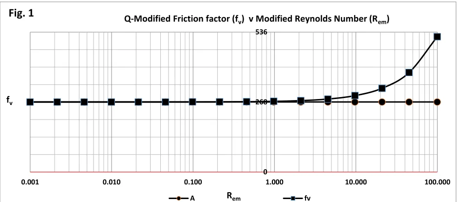
Fig.1 fv is ourQ-modified Ergun type friction factor. A is the constant in our Q-modified Ergun type friction factor. Rem is the modified Reynolds
401
number.
402 403
As shown in Fig. 1, the numerical value of fv and A are virtually identical (268) at values of the
404
modified Reynolds number close to zero and deviate increasingly as the value of fv increases
405
continuously with the value of the modified Reynolds number, above the value of unity. 406
407
Giddings’ Empirical Validation of the Value of 268 for KC
408 409
We focus our attention now on arguably the most important work relating to fluid flow in 410
packed chromatographic columns, which is the now famous first text book of J.C Giddings 411
published in 1965 [33]. At page 198 of the text book, in a footnote, he teaches; “It is impossible 412
to make an absolute distinction between inter-particle and intra-particle free space in 413
connection with flow. All inter-particle space is not engaged in flow because the velocity 414
approaches zero at all solid surfaces and at certain stagnation points. Conversely, all intra-415
particle space is not totally impassive to flow”. Further on in the text, at page 208, when 416
discussing packed bed permeability in the context of the Kozeny-Carman equation, Giddings 417
further opines in relation to the precise value of the constant in that equation; “If it is assumed 418
that for f0 = 0.4, this equation yields ’ = 202. The empirical value, as mentioned earlier, is closer
419
to 300. The same magnitude of discrepancy has been noted by Bohemen and Purnell and by dal 420
Nogare and Juvet for gas chromatographic supports. Hence the factor 300 would appear to be 421
quite reasonable for most chromatographic materials with f0∿ 0.4” (emphasis added). We note
422
that Giddings’ nomenclature for f0 corresponds to our nomenclature of 0, which represents the
423
external porosity of a packed column. Accordingly, Giddings identifies (in 1965) a basic 424
boundary condition of permeability in packed columns by defining the value of his ’ parameter 425
to be 300 when the external porosity of the chromatographic column under study, 0, is 0.4
426 427
By announcing the revised value of 300 for his ’ parameter, Giddings was clearly rejecting the 428
previously accepted lower value of 202 corresponding to the value of 180 for KC, the constant in
429
0 268 536
0.001 0.010 0.100 1.000 10.000 100.000
fv
Rem
Q-Modified Friction factor (fv) v Modified Reynolds Number (Rem)
A fv
the Kozeny/Carman equation [34], an assertion which he says was clearly supported by four 430
other authors in the field of gas chromatography as far back as 1965. This adjustment in the 431
value of his ’ parameter amounts to an increase of a factor of 1.5 (300/202 = 1.5) which when 432
applied to Carman’s identified value of 180 in Giddings’ equation (5.3-10), corresponds to the 433
new value of 267 (180x1.5 = 267). Accordingly, since this Giddings modified value for the 434
Kozeny-Carman constant was first disclosed in 1965, it is of a more recent vintage than either 435
Carman’s value of 180, derived in 1937, or the even more recent value of 150 derived by Ergun 436
in 1952. For an in depth analysis of the basis upon which we believe that Giddings got it right 437
and that this adjustment is justified, see the paper by H.M. Quinn [35]. 438
439
In order to comprehend fully the ramifications of Giddings’ teaching for his ’ parameter and to 440
demonstrate that his experimental results validate our value of 268 for KC, we must take a
441
closer look at how Giddings’ nomenclature for terms and experimental protocols lines up with 442
ours. In order to connect the dots, therefore, between his methodology and ours, we include 443
herein in our Table 1 an elaboration of Giddings’ Table 5.3-1 on page 209 of his 1965 textbook 444
which contains his reported experimental results. 445
446
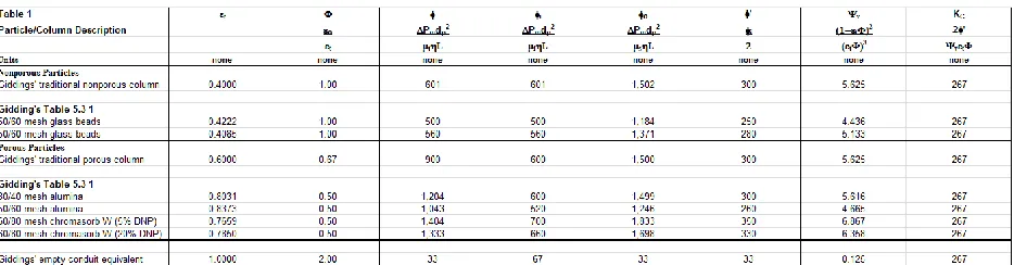
447
Table 1 This Table represents an elaboration of Giddings’ Table 5.3-1 published in his 1965 text book.
448 449
Giddings eliminated the uncertainty of the measurement of external porosity, 0, in columns
450
packed with porous particles by employing the chromatographic technique of injecting small 451
unretained solutes into his packed columns under study. This measurement technique resulted 452
in an accurate value for t, the total porosity of a column packed with porous particles, but it
453
also provided an accurate value for the external porosity, 0, when the particles in the column
454
were nonporous. 455
456
The term t, in our nomenclature, is defined as;
457 458
t =i (28)
459 460
Wheret = the conduit total porosity and,i is defined, in turn, as;
461 462
i =Vi (29)
Vec
464 465
Wherei = the conduit internal porosity and Vi = the cumulative pore volume of all the particles.
466 467
Let us define the term 0, alternatively, in the context of Giddings’ experimental permeability
468
methodology: 469
470
=pack( Spv+1/sk) (30)
471 472
pack = Mp (31)
473
Vec
474 475
Where, pack = the column packing density; Mp =mass of particles in a given column; Spv = the
476
specific pore volume of the particles, sk = the skeletal density of the particles.
477 478
Let us now derive the definition for particle porosity, as follows: 479
480
p = Spvpart (32)
481 482
Where, p = the particle porosity; part = the apparent particle density;
483 484
In order to identify the value of 0 in columns packed with porous particles, Giddings did not
485
rely directly on chromatographic measurements of column external porosity. Rather he used 486
the independently determined value of the particle porosity,p, and supplemented his
487
measured value for t with gravimetric measurements of the amount of particles packed into
488
each column. This experimental technique allowed him to identify the value of his 489
parameter, defined as the ratio of both porosity parameters, i.e. =0/t. Moreover, he
490
eliminated the uncertainty of measuring the particle diameter of porous particles, dp, by using
491
well-defined particle sizes (smooth spherical glass beads) of nonporous particles, which he used 492
in combination with his accurately determined values of t (equivalent to 0 in columns packed
493
with nonporous particles) and by the technique of cross- correlating the pressure drops 494
measured in these columns with pressure drops measured in columns containing porous 495
particles with identical particle diameter values, he grounded his permeability conclusions 496
relative to particle size and column external porosity in the bedrock of measurements made 497
with nonporous spherical particles. Thus Giddings’ methodology is based upon the dependent 498
relationship between particle size, dp and column external porosity, 0, through the correlation
499
factor, np, which is the actual number of spherical particle equivalents packed into any given
500
column based upon its value of dp.
502
We can express this relationship algebraically, as follows; 503
504
npdp= Vec(1-0) (33)
505
6 506
507
Where, np = the number of spherical particle equivalents packed into any given column.
508 509
It follows that we may now algebraically express the external porosity,0, as follows;
510 511
0 =1-(2npdp3)/(3D2L) (34)
512 513
In addition, in his studies relating to column permeability, Giddings used the concept of the 514
flow resistance parameter = Pmdp2/tL, rather than the permeability parameter K0. This is
515
significant because his parameter identifies separately the value of the particle diameter, dp,
516
which in contrast, the permeability parameter, K0, does not. The symbol Pm represents his
517
measured values of the pressure drop as opposed to the theoretically calculated value. 518
Accordingly, it is obvious that use of the permeability parameter, K0, would leave the value of
519
the particle diameter, dp, embedded in the measured value of Pm and, in the absence of
520
measuring the mass of particles packed into a given column under study, would not provide the 521
additional degree of intelligence of identifying, simultaneously and independently, the 522
measured values of particle diameter, dp and column external porosity, 0, which is a
523
prerequisite to validate the value of KC from experimental measurements of pressure gradient.
524
On the contrary, Giddings was careful to identify the value of dp independently from
525
measurements of pressure differential, thus setting a reference value against which he titrated 526
his measurement technique for column resultant porosity following the Laws of Continuity. 527
528
Thus, Giddings was ahead of his peers in using a fundamentally superior technique for defining 529
the components of permeability and, accordingly, he was able to identify the correct value of 530
the embedded constant, Kc, which was something that eluded his peers. For instance, Istvan
531
Halasz, one of Giddings’ most well respected peers, took a decidedly different approach to 532
identifying the fundamentals of permeability. Because of the difficulty of measuring precisely 533
the particle size of irregular silica particles, Halasz made the startling proclamation that the 534
particle size is defined by the permeability [36]. In so doing, unlike Giddings, he essentially 535
buried his head in the sand relative to particle size and adapted the teaching that one ought to 536
start with an assumption relative to the value of Kc and use the Kozeny/Blake equation to
back-537
calculate for the value of the particle size, using Carman’s value of 180 for its constant. The 538
problem with this approach, unfortunately, is that Carman’s value of 180 was erroneously 539
the hat” relative to the value of KC, which is a practice that his disciples have continued to this
541
very day [44] p. 85. 542
543
By using his resistance parameter methodology in his permeability studies of packed columns, 544
however, Giddings had to content with the reality that his measurement of column total 545
porosity, t, resulted in his identification of the mobile phase velocity, t, which in the case of
546
columns packed with porous particles was a major complicating factor relative to third party 547
empirical permeability equations, such as Poiseuille’s for flow in an empty conduit and 548
Kozeny/Carman for flow in a packed column, in as much as it contains a contribution from 549
molecular diffusion within the stagnant pores of the particles, which is not driven by pressure 550
differential. Accordingly, since the aforementioned third party equations were both defined 551
based upon the use of superficial fluid velocity, s, with a corresponding flow resistance 552
parameter = Pmdp2/sL, he was forced to come up with a frame of reference which
553
would connect his methodology to theirs. Moreover, on the one hand, there was the additional 554
complicating factor that the actual velocity that exists in a packed column is neither the mobile 555
phase nor the superficial but rather the interstitial fluid velocity, i, with yet another 556
corresponding flow resistance parameter i = Pmdp2/iL but conversely, on the other hand,
557
interstitial velocity does not ever exist in an empty conduit, which always contains the 558
superficial velocity. This means that he had to invent a methodology which would enable an 559
apples-to-apples comparison between permeability in all flow embodiments at a comparable 560
velocity frame, i.e. interstitial velocity, i, which is the only fluid velocity frame that actually
561
exists in packed conduits when pressure drops are recorded and, superficial velocity,s, which
562
is the only fluid velocity frame that actually exists in empty conduits when pressure drops are 563
recorded and, the remaining mobile phase velocity, which is not a fluid velocity term at all, but 564
rather the velocity of a small unretained solute which penetrates the inner pore volume of the 565
particles in the column, a mechanism driven by solute concentration, not pressure gradient. 566
567
Therefore, Giddings devised a specifically tailored definition of his dimensionless flow 568
resistance parameter, to which he gave the symbol ’, and which would render an approximate 569
constant value no matter what combination of fluid velocity, (s, i, t), particle porosity type
570
(porous, nonporous) or conduit type (packed or empty) a practitioner wanted to employ. 571
572
Accordingly, his ’ parameter represents the dimensionless “constant” in Giddings’ equation 573
which can be applied to a wide variety of different experimental protocols and can include any 574
one of the three distinctly different types of fluid linear velocity encountered in the study of 575
packed conduits containing either porous or nonporous particles, on the one hand, and empty 576
conduits, which contain no solid particles at all, on the other hand. Although its value varies 577
somewhat between 250 and 350 for the packed columns reported in his Table 5.3-1, it does 578
represent a meaningful benchmark within the context of permeability in packed 579
chromatographic columns, to the extent that it incorporates a great variety of particle types, 580
582
As can be seen from our Table 1 herein, our elaboration of Giddings Table 5.3-1 contains our 583
supplemental definitions for Giddings’ terms, which ties together his measured results with his 584
reported values for his ’ parameter for his nonporous glass beads as well as his porous 585
particles of Alumina and Chromasorb. 586
587
Note in particular, that we have included at the bottom of our Table 1 a line item labeled 588
“Giddings’ empty conduit equivalent” which has a ’ value of 33. This clarifies the meaning of 589
his ’ parameter with respect to an empty conduit, inasmuch as it identifies it as our Poiseuille’s 590
type friction factor and confirms that, just as we have independently concluded herein, 591
Giddings had also concluded in 1965 that the numerical value of 32 contained in Poiseuille’s 592
equation is just a little too low to correlate accurately empirical data. This line item in the Table 593
also identifies the correlation coefficient for an empty conduit, v = 0.125, which relates a
594
Poiseuille’s type friction factor and a Kozeny/Carman type friction factor. Therefore, Giddings’ 595
use of his ’ parameter normalized all fluid velocities in an apples-to-apples comparison to that 596
in an empty conduit in which the value of 0 = ’= KP, i.e. the “constant” in Poiseuille’sfluid flow
597
model. 598
599
Note also, as shown in our Table 1, that Giddings’ methodology of using his ’ parameter to 600
identify the value of Kc, does not require the identification of the value of o by itself, but
601
includes it in the ratio, which is his parameter. When the particles are nonporous, on the one 602
hand, this ratio is unity and so measuring t by itself is sufficient to define the value of When
603
the particles are porous, on the other hand, one simply back-calculates for the value of 0 by
604
using his ’ parameter, in order to correlate the measured data, and, thus, establish the value of
605
0 embedded in the value of . Therefore, Giddings’ methodology, in the case of porous
606
particles, is in conformance with the Laws of Continuity to the extent that he uses the value of, 607
dp, which has been measured independently of the column under study and the INDEPENDENT
608
measurement of both particle porosity, p, and the mass of the particles, Mp, packed into any
609
given column. He assigns his independently measured value of dp as his independent column
610
variable and the value of, 0, as his dependent column variable. Accordingly, by the use of his ’
611
parameter, Giddings’ also found a way to “engineer” around the difficulty of measuring 612
accurately the value of external porosity, o, in columns packed with porous particles, without
613
putting a rabbit in the hat with respect to the value of KC, as was the method chosen by Halasz 614
to solve his unique dilemma, a direct consequence of choosing to work with irregularly shaped 615
particles, in the first instance. 616
617
Finally, as is also apparent in our Table 1, the value of 267 for KC which represents our
Q-618
modified Ergun viscous type friction factor (also the modified Kozeny/Carman type friction 619
factor) compares favorably to our independently asserted value of 268. 620
621
The major objectives of the experimental protocol outlined in this paper are to: 624
a. Design a fluid flow experiment which meets the standards of a properly configured 625
fluid dynamics experiment, i.e. all contribution to energy dissipation is captured. 626
b. Minimize/eliminate any and all uncertainty related to the experimental variables of 627
particle diameter, dp, and packed bed external porosity, 0.
628
c. Validate empirically the value of the Kozeny/Carman constant, i.e. the remainder in 629
this empirical equation after all measurable entities have been accounted for. 630
631
Since a major source of the uncertainty in the value of KC relative to modern day HPLC packed
632
columns has to do with the accurate measurement of diameter of fully porous particles, dp, and
633
a determination of the column external porosity, 0, two critical parameters involved in the
634
determination of packed column permeability, we use empty conduits (capillaries) in our 635
experiments to eliminate this particular issue. In this way, we replace the difficult-to-measure 636
diameter of fully porous particles, typically less than 2 microns in modern day UHPLC columns, 637
with that of the diameter of a capillary which is several orders of magnitude greater in 638
characteristic dimension. In addition, we use capillaries of different lengths in conjunction with 639
various fluids of varying viscosity to further insure the integrity of our measured values. By 640
invoking the well-known/established Poiseuille’s flow model for empty conduits, which does 641
not possess a porosity term on its face, (porosity being embedded in the “constant” value of 642
33), we “engineer” a way around the uncertainty associated with the measurement of porosity 643
in packed columns. Once we establish the value of the residual constant in empty conduits in 644
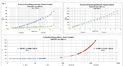
which we have minimized the uncertainty associated with the measurements of characteristic 645
dimension and conduit porosity, we use it as a “given” when we turn our attention to packed 646
conduits wherein we avoid the use of small, fully porous particles in favor of large, nonporous 647
particles which will, once again, minimize the uncertainty associated with the measurement of 648
650 651
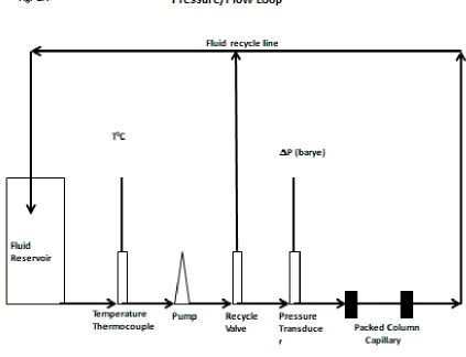
Fig. 2A Pressure/Flow loop used in our experiments to determine the permeability of empty and packed conduit
652 653
In Fig. 2A we show a schematic block diagram of the experimental apparatus that we used to 654
measure the permeability in both empty and packed conduits. In every experiment, we 655
measured the temperature, flow rate and pressure drop at as many flow rates as was 656
reasonably possible given the constraints of the pump, i.e. maximum pressure, minimum flow 657
rate and pump power. The pressure drop was recorded by means of a calibrated pressure 658
transducer purchased from Omega, Model # PX409-250DWU5V. It had a pressure range of 0-659
250 psi and run under a 24V DC power supply. The flow rate was measured for each recorded 660
pressure drop by means of a stop watch and graduated cylinder. The time interval over which 661
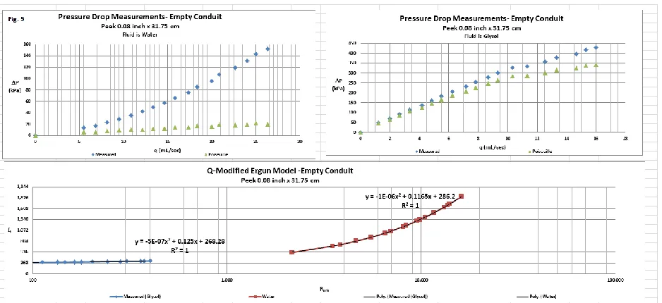
the measurement was taken varied with the flow rate-larger for low flow rates and smaller for 662
high flow rates. The temperature of the fluid was recorded by means of a thermocouple 663
purchased from Omega, Model # TCK-NPT-72. 664
665
The liquid pump was manufactured by Fluid-o-Tech (Italy), Model # FG204XDO(P.T)T1000. It is 666
under a software control package manufactured by National Instruments. The pump had a flow 669
rate range of 100-1600 mL/min and a pressure maximum rating of circa 200 psi. This range of 670
flow rates was further enhanced at lower flow rate values by the use of our recycle valve, which 671
was used to shunt the flow between the devise under study and the recycle line. 672
673
The Air pump was a 3L Calibrated Syringe type pump manufactured by Hans Rudolf Inc., 674
Shawnee, KS, USA., and Model # 5630, serial # 553. 675
3 3. Results and discussion 676
677
3.1Empty Conduits 678
679
Experiment # 1 680
681
In our experiment # 1, we chose to evaluate the permeability of a commercially available empty 682
capillary made of Peek plastic, an article of commerce in the HPLC industry, which had a 683
nominal diameter of 0.02 inches. We chose to evaluate two different lengths, 100 cm and 726 684
cm, in order to be able to exploit different modified Reynolds number ranges of the fluid flow 685
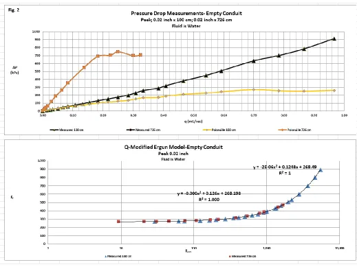
regime and we have captured our results in Fig.2. 686
688 689
Fig. 2The measured results for flow capillary with dimensions 0.02 inches in diameter and 100 and 726 cm in length. The upper plot is the
690
results in dimensional format plotted as flow rate versus pressure drop. The lower plot is the Q-modified Ergun type friction factor plotted as
691
modified Reynolds number versus friction factor.
692 693
As can be seen from Fig.2 in the dimensional plot, Poiseuille’s equation, as expected, deviates 694
increasingly from the measured results as the flow rate increases. In the dimensionless plot in 695
Fig. 2, we show a plot of fv on the y axis and Rem on the x axis. Using a logarithmic scale on the
696
x-axis and a quadratic equation of the line for the measured data, we demonstrate that the 697
intercept on the y-axis for the measured data is 268 (approx.) for both capillaries. Finally, as 698
also shown on the dimensionless plot, the Poiseuille’s equation does not correlate the 699
measured data at the higher Reynolds number values and is slightly too low, even at the 700
lowest values of the modified Reynolds number. 701
702
Experiment # 2. 703
fluids, water and Glycol, and captured the measured results in Fig. 3. The viscosity of the 707
water was 0.01poise and the density was 1.0 g/mL. The viscosity for the Glycol solution was 708
0.38poise and the density was 1.14 g/mL. 709
710
711 712
Fig. 3 The measured results for flow capillary with dimensions 0.03 inches in diameter and 100 and 700 cm in length. The upper plot is the
713
results in dimensional format plotted as flow rate versus pressure drop. The lower plot is the Q-modified Ergun type friction factor plotted as
714
modified Reynolds number versus friction factor.
715 716
As can be seen from Fig.3, by including the measurements in the higher viscosity fluid, Glycol, 717
we are able to focus on the deviations of the Poiseuille’s model at lower modified Reynolds 718
number values. This experiment again identifies the universal value of the residual constant as 719
268 under all measurement conditions. 720
721
Experiment #3. 722
723
In our experiment # 3, we chose a stainless steel capillary of nominal diameter 0.07 inches x 724
726
Fig. 4 The measured results for flow capillary with dimensions 0.07 inches in diameter and 66.5 cm in length. The upper plot is the results in
727
dimensional format plotted as flow rate versus pressure drop. The lower plot is the Q-modified Ergun type friction factor plotted as modified
728
Reynolds number versus friction factor.
729 730
As shown in Fig. 4, the results for this simple one length capillary shows that a practitioner 731
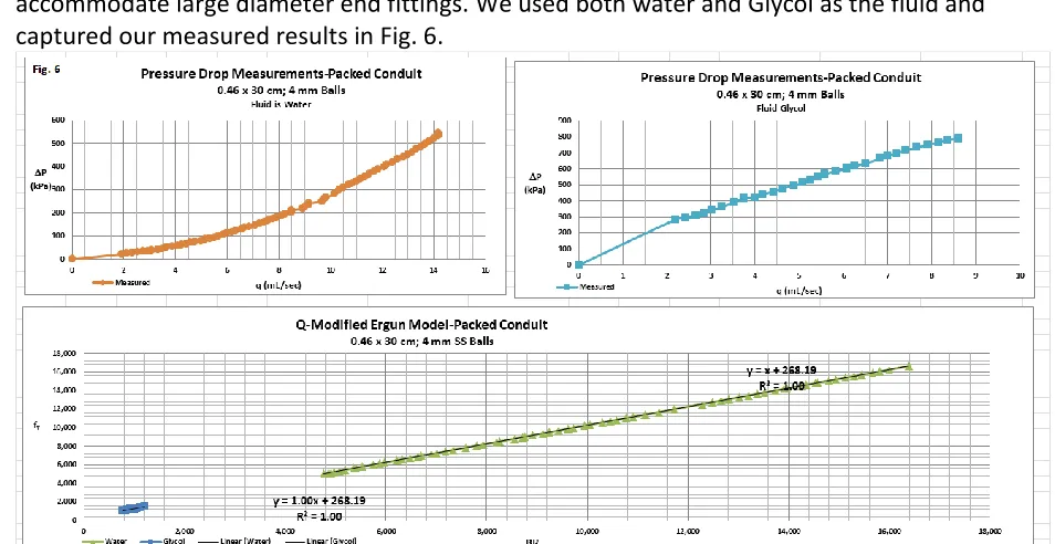
may use it in conjunction with Glycol as the fluid to easily demonstrate the universal value of 732
268 for the residual constant. This experiment also teaches the practitioner that the intercept 733
is sensitive to the range of Reynolds number covered in the measurements- as shown in the 734
plot an intercept value of 281 represents a higher range of Reynolds numbers. 735
736
Experiment #4. 737
738
In our experiment # 4, we chose a stainless steel capillary of nominal diameter 0.08 inches x 739
741
Fig. 5 The measured results for flow capillary with dimensions 0.08 inches in diameter and 31.75 cm in length. The upper plot is the results in
742
dimensional format plotted as flow rate versus pressure drop. The lower plot is the Q-modified Ergun type friction factor plotted as modified
743
Reynolds number versus friction factor.
744 745
As shown in Fig. 5, the results for this simple one length capillary shows that a practitioner 746
may use it in conjunction with Glycol and water as the fluid to easily demonstrate the 747
universal value of 268 for the residual constant. 748
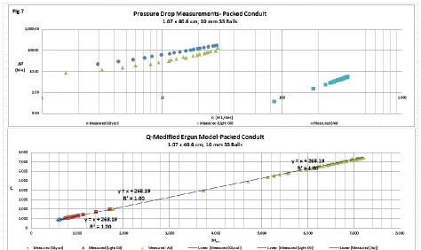
749
3.2Packed Conduits 750
751
In our experiments with packed conduits, we wanted to eliminate issues related to the accuracy 752
of measuring particle size and packed column external porosity. We accomplished this by using 753
very large electro-polished (smooth) stainless steel non porous ball bearings. In addition, by 754
counting the number of particles in each packed column (76 in one case and 45 in the other) 755
and by knowing the exact volume of each particle, we were able to eliminate any uncertainty 756
relating to external column porosity. This particular choice of experimental variables means 757
that our packed columns had extraordinarily high values of external porosities and 758
correspondingly low values for column to particle diameter ratios, from a chromatographic 759
column utility point of view. However, although such packed columns may not be of great 760
utility in solving modern day separation problems, there is nothing unusual about these packed 761
columns from a hydrodynamic point of view and, accordingly, they easily overcome our 762
experimentally challenging permeability objectives from an accuracy of measurement point of 763
view. Another consequence of this set of experimental variable choices, however, is that our 764
measurements have to be made at relatively high values of the modified Reynolds number, 765
where kinetic contributions play a dominant role in the overall contributions to measured 766
pressure drop. Accordingly, in order to experimentally identify the value of A in this flow 767
regime, we must normalize our measured pressure drops for kinetic contributions which dictate 768
that we must first identify the value of B in our dimensionless manifestation of the Q-modified 769
Ergun viscous type friction factor. 770
We begin by repeating our equation (25) which represents the friction factor in the Q-modified 772
Ergun viscous type friction factor; 773
774
fv = + Rem (25)
775 776
We now make use of our determination of the value of 268 for A above, by substitution this 777
numerical value into equation (25). Thus we may write: 778
779
fv = + Rem (35)
780 781
Rearranging equation (35) to isolate the value of B gives: 782
783
fv-268 = (36)
784
Rem
785 786
Since we have experimentally measured every variable on the left hand side of equation (36) 787
for each data point in our study, we can calculate the value of B corresponding to each recorded 788
pressure drop by using equation (36). Accordingly, the value of B represents a lumped 789
parameter which, when combined with the value of the modified Reynolds number, contains all 790
the individual kinetic contributions, whatever they may be. We can now further exploit the 791
relationship in equation (25) to determine the value of A in any experimental packed column 792
under study. To accomplish this objective we make a plot of fv on the y axis and BRem on the x
793
axis and using a linear equation as a fit to the measured data in the experimental column, we 794
can identify the value of A as the intercept on the y axis. This procedure normalizes for kinetic 795
contributions by setting the slope of the straight line in this plot equal to unity. 796
797
In reality, therefore, in the case of a packed conduit, our methodology to identify the value of A 798
normalizes the flow term for kinetic contributions in the non-linear component of the pressure 799
flow relationship. This is in contrast to our methodology to identify the value of A in an empty 800
conduit, which normalizes the pressure drop term for viscous contributions in the linear 801
component of the pressure flow relationship. Accordingly, our methodology is orthogonal with 802
respect to its identification of the value of A in empty and packed conduits, respectively, as well 803
as in laminar and non-laminar flow regimes, respectively. 804
805
Experiment # 5. 806
807
In our experiment number 5, we placed 76, nominal 4 mm stainless steel perfectly spherical ball 808
bearings into a 0.46 x 30 cm peek column. The particles were touching each other at a single 809
accommodate large diameter end fittings. We used both water and Glycol as the fluid and 811
captured our measured results in Fig. 6. 812
813
Fig. 6 The measured results for the packed conduit with dimensions 0.46 cm diameter and 30 cm in length. The upper plot is the results in
814
dimensional format plotted as flow rate versus pressure drop. The lower plot is the Q-modified Ergun type friction factor plotted as normalized
815
modified Reynolds number versus friction factor.
816 817
The measured external porosity of the column, 0, was 0.499 and the value of the particle
818
diameter, dp, was 3.975 mm. As can be seen in the dimensionless plot in Fig. 6, the data points
819
in both lines representing the measured data fall on a straight line of slope unity and intercept 820
268, thus validating the value of A. 821
822
Experiment # 6. 823
824
In our experiment number 6, we used two different values of external porosity in the 825
experiment. The column that we used with air as the fluid had 41 particles and the other 826
column which we used with both light oil and glycol had 45 particles. These particles were 827
nominal 10 mm stainless steel perfectly spherical ball bearings in a 1.07 x 40.6 cm stainless 828
steel column. The particles were touching each other at a single point in the packed column 829
array. The column end-fittings were custom-drilled to accommodate large diameter end 830
fittings. We used both light oil and Glycol as the fluid in one column and air as the fluid in the 831
other and we captured our measured results in Fig. 7. In the experiments with the light oil, we 832
used the value of 0.153poise, for the absolute viscosity of the fluid, and a value of 0.80 g/mL for 833
835
Fig. 7 The measured results for the packed conduit with dimensions 1.07 cm diameter and 40.6 cm in length. The upper plot is the results in
836
dimensional format plotted as flow rate versus pressure drop. The lower plot is the Q-modified Ergun type friction factor plotted as normalized
837
modified Reynolds number versus friction factor.
838 839
The measured external porosity of this larger volume column, 0, was 0.44 corresponding to
840
the column with 45 particles, and 0.49 corresponding to the column which contained the 41 841
particles. The value of the particle diameter, dp, was 9.525 mm. As can be seen in Fig. 7 the
842
data points in all three lines representing the measured data fall on a straight line of slope 843
unity and intercept 268, thus validating the value of A. 844
845
3.3Third Party Independent Validation of experimental Protocol 846
847
Whenever one seeks to challenge conventional wisdom, as we are doing in this paper, one 848
must be vigilant to guard against criticism of all different kinds. In order to defend our 849
methodology against those who may suggest that it is based solely upon measurements made 850
in our own laboratory, which is true, and consequently may not be repeatable or reproducible, 851
which is not true, we look to validate using independent means. To this end we include in this 852
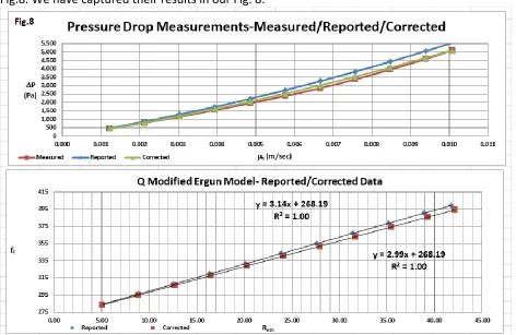
section the experiment of Sobieski and Trykozko published relatively recently (2014)[38]. 853
854
In their experiment, they used non porous smooth spherical glass beads of diameter 1.95 mm. 855
Their column was 90 cm in length and 8 cm in diameter. Accordingly, the empty column volume 856
was about 4.5 L, all of which translates into very manageable measurements from an accuracy 857
Table 1 and 2 in the paper as well as providing a plot of pressure drop against fluid velocity in 860
Fig.8. We have captured their results in our Fig. 8. 861
862
Fig. 8 Experimental results of Sobieski et al. Upper plot is pressure drop against velocity. Lower plot is dimensionless plot of fv against Rem
863 864
We point out initially that the experimental design parameters in this experiment represent a 865
“special case” of our teaching protocol herein, to the extent that the measurements were all 866
taken over a range of modified Reynolds numbers in which the value of B is virtually constant. 867
Accordingly, we may use a linear regression analysis in our plot of fv against Rem to validate both
868
components of our methodology, i.e. validate the value of A and identify the correct value of 869
the kinetic coefficient, B. As is shown in Fig 8, in the dimensional plot, the measured pressure 870
drop values do not line up exactly with the calculated pressures based upon the reported 871
underlying variables. In the dimensionless plot, the reported underlying variables validate the 872
value of 268 for A and a value of 3.14 for B. This value of B is not accurate, however, because it 873
does not correlate the data perfectly, especially at the higher values of the modified Reynolds 874
number. We have adjusted the value of 0, reported as 0.37, to the value of 0.376 in order to
875
correlate the measured data. This represents an increase of 1.7% in the value of 0. The
876
corrected data in the dimensionless plot, which correlates the measured values perfectly, 877
generates a value of 2.99 for B which is a decrease of 4.8%. 878
879
Accordingly, our protocol outlined in this paper, when applied to the experiment of Sobieski et 880
al, validates the value of 268 for A and a value of 2.99 for B, with an uncertainty of less than 2% 881
in the value of the external porosity, 0, and less than 5% in the value of B.
4. Some Worked Examples. 884
885
Now that we have disclosed a methodology to enable a practitioner to identify the value of A 886
in a packed column, let us demonstrate the utility of the teaching from the perspective of a 887
potential researcher who wants to use it to evaluate the credibility, or lack thereof, of third 888
party published permeability experiments. 889
890
Example 1. 891
892
In this example, we evaluate our own measured permeability results for column number 893
HMQ-2 which was manufactured circa the year 2000, approximately 18 years ago, in the 894
author’s laboratory in Franklin, Ma. This column consisted of a stainless steel column 248 cm 895
(8 ft.) in length and 1.002 cm in diameter. The column was manufactured by placing the 896
empty conduit upright in a holding devise and this author, by means of a step ladder, placed 1 897
mm diameter spherical glass beads into the column by pouring the dried beads into the 898
column slowly, while at the same time, vibrating the column with a hand-held mechanical 899
vibrator, a typical dry-packing technique well-known in conventional HPLC circles. After the 900
column was filled with the glass beads, water was poured into the column slowly until it 901
overflowed. The amount of water in took to fill the column (76 ml) represents the volume of 902
fluid external to the particles in the packed column and, when divided by the empty column 903
volume of 196 mL, results in an external porosity value, 0, for this nonporous particle column,
904
of 0.39. The choice of this large internal volume column in combination with nonporous glass 905
beads of 1 mm nominal diameter, was driven by the design objective to, once again, minimize 906
the measurement uncertainty in the measured values of particle diameter, dp, and column
907
external porosity, 0. We used a preparative HPLC pump, manufactured by Ranin Corp., to
908
flow water through the column and the pressure drops were measured by means of a 909
calibrated pressure transducer over a flow rate range of 300 to 500 mL, approx. We have 910
912
Fig. 9 The measured results for column HMQ-2. The upper plot is the results in dimensional format plotted as flow rate versus pressure drop.
913
The lower plot is the Q-modified Ergun type friction factor plotted as normalized modified Reynolds number versus friction factor.
914 915
As can be seen from Fig.9 the measured data points on the dimensionless plot all fall on a 916
straight line of slope unity and intercept 268 which validate the value of A. 917
918
Example 2. 919
920
In this example, we examine a published scientific article in the Journal of Chromatography by 921
Cabooter et al (2008) [39]. This publication represents one example of what we have referred 922
to above regarding the value of the Kozeny/Carman constant, KC, being used as a tool to
923
justify false separation performance claims pertaining to the modern chromatography 924
columns containing the so-called sub 2 micron particles. In this paper, the authors report 6 925
different values for KC supposedlybased upon their experimental assessment of 6 different
926
commercially available chromatographic columns. We will use our methodology disclosed 927
herein, however, to demonstrate that, not only did the authors not experimentally validate 928
their erroneous values for KC by using credible scientific principles, but also, the values of their
929
underlying combinations for the parameters of dp and 0, are demonstrably false. In our Fig.
930
10 herein, we have captured the authors’ reported results and applied our methodology 931
reported herein to demonstrate that, not only is our teaching herein effective in identifying 932
substandard scientific publications, but also, it can be used effectively to correct the reported 933
data and present a true picture of what the experimental results really identify as the 934
936
Fig. 10 The measured results for the Cabooter et al paper. The upper plot is the results in dimensional format plotted as flow rate versus
937
pressure drop. The lower plot is the Q-modified Ergun type friction factor plotted as normalized modified Reynolds number versus friction
938
factor.
939 940
As can be seen in the dimensionless plot in Fig. 10 representing the reported results, the 941
values of fv on the y axis are identical to the values of KC reported by the authors for each of
942
the 6 columns, but when their reported modified Reynolds numbers values are normalized for 943
kinetic contributions on the x axis, the intercept of the straight line has a value of 268, thus 944
validating the true value of KC. However, all the plotted values on the x axis are negative (less
945
than zero). On the other hand, as can also be seen in the dimensionless plot in Fig. 10 946
representing the corrected results, all 6 values of fv on the y axis have the same value of 268
947
and all the corresponding modified Reynolds number values when normalized for kinetic 948
contributions on the x axis, are positive (greater than zero). We have also included in Fig. 10, a 949
dimensional plot of the measured pressure drop versus fluid flow rate for both the reported 950
results as well as our corrected results to demonstrate that our correction methodology does 951
not alter any of the measured values which are not subject to measurement uncertainty. 952
953
The only scientifically valid explanation for the negative values of BRem on the x axis for the
954
reported results is that the fluid in the column was moving backwards against the pressure 955
gradient when the pressure drops were recorded within the column, a phenomenon which all 956
knowledgeable scientists will agree is physically impossible. Accordingly, we know that the 957
values of the modified Reynolds numbers derived based upon the reported results are in 958
error. Since the modified Reynolds number parameter is comprised only of 5 discrete 959
variables, s, dp, f, o, and , all of which values we do not question except, dp ando, we
960
conclude thatthe combination of these two variables reported by the authors for each of the 961