Quantum Minimum Distance Classifier
Enrica Santucci
1 University of Cagliari, Piazza D’Armi snc - 09123 Cagliari (Italy); [email protected]
Abstract:We propose a quantum version of the well known minimum distance classification model
1
calledNearest Mean Classifier(NMC). In this regard, we presented our first results in two previous
2
works. In [34] a quantum counterpart of the NMC for two-dimensional problems was introduced,
3
namedQuantum Nearest Mean Classifier(QNMC), together with a possible generalization to arbitrary
4
dimensions. In [33] we studied the n-dimensional problem into detail and we showed a new
5
encoding for arbitrary n-feature vectors into density operators. In the present paper, another
6
promising encoding ofn-dimensional patterns into density operators is considered, suggested by
7
recent debates on quantum machine learning. Further, we observe a significant property concerning
8
the non-invariance by feature rescaling of our quantum classifier. This fact, which represents a
9
meaningful difference between the NMC and the respective quantum version, allows to introduce a
10
free parameter whose variation provides, in some cases, better classification results for the QNMC.
11
The experimental section is devoted to:i)compare the NMC and QNMC performance on different
12
datasets;ii)study the effects of the non-invariance under uniform rescaling for the QNMC.
13
Keywords:quantum formalism applications; minimum distance classification; rescaling parameter
14
1. Introduction 15
In the last few years, many efforts to apply the quantum formalism to non-microscopic contexts
16
have been made [1,24,26,32,37,41]. The idea is that the powerful predictive properties of quantum
17
mechanics, used for describing the behavior of microscopic phenomena, turn out to be particularly
18
beneficial also in non-microscopic domains. Indeed, the real power of quantum computing consists in
19
exploiting the strength of particular quantum properties in order to implement algorithms which are
20
much more efficient and faster than the respective classical counterpart. At this purpose, several non
21
standard applications involving the quantum mechanical formalism have been proposed, in research
22
fields such as game theory [8,27], economics [11], cognitive sciences [2,40], signal processing [9], and
23
so on. Further, particular applications, interesting for the specific topics of the present paper, concern
24
the areas of machine learning and pattern recognition.
25
Quantum machine learning is an emerging research field which can use the advantages of
26
quantum computation in order to find new solutions to pattern recognition and image understanding
27
problems. About this, some attempts which connect quantum information to pattern recognition can
28
be found in [31], while an exhaustive survey and bibliography of the developments regarding the use
29
of quantum computing techniques in artificial intelligence are provided in [23,45].
30
In this context, there exist different approaches involving the use of quantum formalism in
31
pattern recognition and machine learning. We can find for instance procedures which exploit quantum
32
properties without presupposing the help of a quantum computer [13,19,38] or techniques supposing
33
the existence of a quantum computer in order to perform in an inherently parallel way all the required
34
operations, taking advantage of quantum mechanical effects and providing high performance in terms
35
of computational efficiency [5,28,44].
36
One of the main aspects of pattern recognition is focused on the application of quantum
37
information processing methods [20] to solve classification and clustering problems [5,12,39].
38
The use of quantum states for representing patterns has a twofold motivation: as already
39
discussed, first of all it gives the possibility of exploiting quantum algorithms to boost the
40
computational efficiency of the classification process. Secondly, it is possible to use quantum-inspired
41
models in order to reach some benefits with respect to classical problems.
42
Even if the state-of-art approaches suggest possible computational advantages of this sort [3,21,22],
43
the main problem to find amore convenientencoding from classical to quantum objects is nowaday
44
an open and interesting matter of debate [23,31]. Here, our contribution consists in constructing a
45
quantum version of a minimum distance classifier in order to reach some convenience, in terms of
46
the error in pattern classification, with respect to the corresponding classical model. We have already
47
proposed this kind of approach in two previous works [33,34], where a “quantum counterpart” of the
48
well knownNearest Mean Classifier(NMC) has been presented.
49
In both cases, the model is based on the introduction of two main ingredients: first, an appropriate
50
encoding of arbitrary patterns into density operators; second, a distance measure between density
51
operators, representing the quantum counterpart of the Euclidean distance in the “classical” NMC.
52
The main difference between the two previous works is the following one: i)in the first case [34],
53
we tested our quantum classifier on two-dimensional datasets and we proposed a generalization to
54
arbitrary dimension from a theoretical point of view only;ii)in the second case [33], a new encoding
55
for arbitraryn-dimensional patterns into quantum states has been proposed, and it was tested on
56
different real-world and artificial two-class datasets. Anyway, in both cases we observed a significant
57
improvement of the accuracy in the classification process. In addition, we found that, by using the
58
encoding proposed in [33] and for two-dimensional problems only, the classification accuracy of our
59
quantum classifier can be further improved by performing a uniform rescaling of the original dataset.
60
In this work we propose a new encoding of arbitraryn-dimensional patterns into quantum
61
objects, extending both the thoretical model and the experimental results to multi-class problems,
62
which preserves information about the norm of the original pattern. This idea has been inspired by
63
recent debates on quantum machine learning [31], according to which it is crucial to avoid loss of
64
information when a particular encoding of real vectors into quantum states is considered. Such an
65
approach turns out to be very promising in terms of classification performance with respect to the
66
classical version of the NMC. Further, differently from the NMC, our quantum classifier is invariant
67
under uniform rescaling. More precisely, the accuracy of the quantum classifier changes by rescaling
68
(of an arbitrary real number) the coordinates of the dataset. Consequently, we observe that, for
69
several datasets, the new encoding exhibits a further advantage that can be gained by exploiting the
70
non-invariance under rescaling, also forn-dimensional problems (conversely to the previous works).
71
At this purpose, some experimental results have been presented.
72
The paper is organized as follows: in Section2we briefly describe the classification process
73
and, in particular, the formal structure of the NMC for multi-class problems. Section3is devoted
74
to the definition of a new encoding of real patterns into quantum states. In Section4we introduce
75
the quantum version of the NMC, calledQuantum Nearest Mean Classifier(QNMC), based on the
76
new encoding previously described. In Section5we compare the NMC and the QNMC on different
77
datasets showing that, in general, the QNMC exhibits a better performance (in terms of accuracy and
78
other significant statistical quantities) with respect to the NMC. Further, starting from the fact that,
79
differently from the NMC, the QNMC is not invariant under rescaling, we also show that for some
80
datasets it is possible to provide a benefit from this non-invariance property. Some conclusions and
81
possible further developments are proposed at the end of the paper.1
82
2. Minimum distance classification 83
Pattern recognition [7,43] is the scientific discipline which deals with theories and methodologies
84
for designing algorithms and machines capable of automatically recognizing “objects” (i.e. patterns) in
85
noisy environments.
86
Here, we deal withsupervised learning,i.e.learning from a training set of correctly labeled objects.
87
In other words, this is the case in which examples of input-output relations are given to a computer
88
and it has to infer a mapping from there. The most important task ispattern classification, whose goal is
89
to assign input objects to different classes.
90
More precisely, each object can be characterized by its features; hence, ad-feature object can be
91
naturally represented by ad-dimensional real vector, i.e.~x= [x(1), . . . ,x(d)]∈ X, whereX ⊆Rdis 92
generally a subset of thed-dimensional real space representing thefeature space. Consequently, any
93
arbitrary object is represented by a vector~xassociated to a given class of objects (but, in principle, we
94
do not know which one). LetY ={1, . . . ,L}be the class label set. Apatternis represented by a pair
95
(~x,y), where~xis thefeature vectorrepresenting an object andy∈ Yis thelabelof the class which~xis
96
associated to. The aim of the classification process is to design a function (classifier) that attributes (in
97
the most accurate way) to any unlabeled object the corresponding label (where the label attached to an
98
object represents the class which the object belongs to), by learning about the set of objects whose class
99
is known. Thetraining setis given byStr= {(~xn,yn)}nN=1, where~xn ∈ X,yn ∈ Y(forn= 1, . . . ,N) 100
andNis the number of patterns belonging toStr. Finally, letNlbe the cardinality of the training set 101
associated to thel-th class (forl=1, 2, . . . ,L) such that∑L
l=1Nl=N. 102
We now introduce the well knownNearest Mean Classifier(NMC) [7], which is a particular kind of
103
minimum distance classifier widely used in pattern recognition. The strategy consists in computing the
104
distances between an object~x(to classify) and other objects chosen as prototypes of each class (called
105
centroids). Finally, the classifier associates to~xthe label of the closest centroid. So, we can resume the
106
NMC algorithm as follows:
107
1. computation of the centroid (i.e. the sample mean [15]) associated to each class, whose corresponding feature vector is given by:
~µl=
1
Nl Nl
∑
n=1
~xn, l=1, 2, . . . ,L, (1)
wherelis the label of the class;
108
2. classification of the object~x, provided by:
argminl=1,...LdE(~x,~µl), with dE(~x,~µl) =k~x−~µlk2, (2)
wheredEis the standard Euclidean distance.2. 109
Depending on the particular distribution of the dataset patterns, it is possible that a pattern
110
belonging to a given class is closest to the centroid of another class. In this case, if the algorithm would
111
be applied to this pattern, it would fail. Hence, for an arbitrary object~xwhose class isa prioriunknown,
112
the output of the above classification process has the following four possibilities [10]:i) True Positive 113
(TP): pattern belonging to thel-th class and correctly classified asl;ii) True Negative(TN): pattern
114
belonging to a class different thanl, and correctly classified as notl;iii) False Positive(FP): pattern
115
belonging to a class different thanl, and uncorrectly classified asl;iv) False Negative(FN): pattern
116
belonging to thel-th class, and uncorrectly classified as notl.
117
2 We remind that, given a functionf :X→Y, theargmin(i.e.the argument of the minimum) over some subsetSofXis defined as:argminx∈S⊆Xf(x) ={x|x∈S∧ ∀y∈S: f(y)≥f(x)}. In this framework, the argmin plays the role of the
In order to evaluate the performance of a certain classification algorithm, the standard procedure
118
consists in dividing the original labeled datasetS ofN0patterns, into a training setStrofNpatterns 119
and a setStsof(N0−N)patterns (i.e.S =Str∪ Sts). This setStsof patterns is calledtest set[7] and it 120
is defined asSts={(~xn,yn)}N 0 n=N+1. 121
As a consequence, by applying the NMC to the test set, it is possible to evaluate the classification
122
algorithm performance by considering the following statistical measures associated to each classl 123
depending on the quantities listed above:
124
• True Positive Rate(TPR): TPR= TP+FNTP ;
125
• True Negative Rate(TNR): TNR= TN+FPTN ;
126
• False Positive Rate(FPR): FPR= FP+TNFP =1−TPN;
127
• False Negative Rate(FNR): FNR= FN+TPFN =1−TPR.
128
Further, other standard statistical coefficients [10] used to establish the reliability of a classification
129
algorithm are:
130
• Classification error(E): E=1− TP
N0−N; 131
• Precision(P): P= TP+FPTP ;
132
• Cohen’s Kappa(K): K= Pr(a)1−Pr(e)−Pr(e), where
133
Pr(a)= TP+TNN0−N , Pr(e)= (TP+FP)(TP+FN)+(FP+TN)(TN+FN)(N0−N)2 . 134
In particular, the classification error represents the percentage of misclassified patterns, the
135
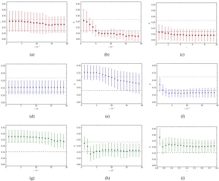
precision is a measure of the statistical variability of the considered model and the Cohen’s Kappa
136
represents the degree of reliability and accuracy of a statistical classification and it can assume values
137
ranging from −1 to +1 (K= +1 corresponds to a perfect classification procedure while K= −1
138
corresponds to a completely wrong classification). Let us note that these statistical coefficients have
139
to be computed for each class. Then, the final value of each statistical coefficient related to the
140
classification algorithm is the weighted sum of the statistical coefficients of each class.
141
3. Mapping real patterns into quantum states 142
As already discussed, quantum formalism turns out to be very useful in non-standard scenarios,
143
in our case to solve for instance classification problems on datasets of classical objects. At this purpose,
144
in order to provide our quantum classification model, the first ingredient we have to introduce is an
145
appropriate encoding of real patterns into quantum states. Quoting Schuld et al. [31], “in order to
146
use the strengths of quantum mechanics without being confined by classical ideas of data encoding,
147
finding ‘genuinely quantum’ ways of representing and extracting information could become vital for
148
the future of quantum machine learning.”
149
Generally, given ad-dimensional feature vector, there exist different ways to encode it into a density operator [31]. In [34], the proposed encoding was based on the use of the stereographic projection [6]. In particular, it allows to unequivocally map any point~r= (r1,r2,r3)on the surface of a radius-one sphereS2(except for the north pole) into an arbitrary point~x= [x(1),x(2)]inR2,i.e.
SP:(r1,r2,r3)7→ r1
1−r3, r2
1−r3
= [x(1),x(2)]. (3)
The inverse of the stereographic projection is given by:
SP−1:[x(1),x(2)]7→h 2x
(1)
||~x||2+1,
2x(2)
||~x||2+1,
||~x||2−1
||~x||2+1
i
where ||~x||2 = [x(1)]2+ [x(2)]2. By imposing thatr1 = 2x(1)
||~x||2+1, r2 = 2x
(2)
||~x||2+1, r3 =
||~x||2−1
||~x||2+1, if we
considerr1,r2,r3as Pauli components3of a density operatorρ~x∈Ω24, the density operator associated
to the pattern~x= [x(1),x(2)]can be written as:
ρ~x=
1 2
1+r3 r1−ir2 r1+ir2 1−r3
!
= 1
||~x||2+1
||~x||2 x(1)−ix(2) x(1)+ix(2) 1
!
. (5)
The advantage in using this encoding consists in the fact that it provides an easy visualization of
150
an arbitrary two-feature vector on the Bloch sphere [34]. In the same work, we also introduced a
151
generalization of our encoding to thed-dimensional case, allowing to express arbitraryd-feature
152
vectors as points on the hypersphereSdby writing a density operatorρas a linear combination of the 153
d-dimensional identity andd2−1(d×d)-square matrices{σi}(i.e. generalized Pauli matrices[4,17]). 154
At this purpose, we introduced the generalized stereographic projection [16], which maps any point~r= (r1, . . . ,rd+1)∈Sdinto an arbitrary point~x= [x(1), . . . ,x(d)]∈Rd,i.e.:
SP:(r1, . . . ,rd+1)7→
r1
1−rd+1
, r2
1−rd+1
, . . . , rd 1−rd+1
= [x(1), . . . ,x(d)]. (6)
However, even if it is possible to map points on thed-hypersphere intod-feature patterns, such points
155
do not generally represent density operators and the one-to-one correspondence between them and
156
density matrices is guaranteed only on particular regions [14,17,18].
157
An alternative encoding of ad-feature vector~x into a density operator was proposed in [33]. It is obtained: i)by mapping~x ∈ Rdinto a (d+1)-dimensional vector~x0 ∈ Rd+1according to the
generalized version of Eq. (4),i.e.
SP−1:[x(1), . . . ,x(d)]7→ 1 ||~x||2+1
h
2x(1), . . . , 2x(d),||~x||2−1i= (r1, . . . ,rd+1), (7)
where||~x||2=∑d
i=1[x(i)]2;ii)by considering the projectorρ~x=~x0·(~x0)T. 158
In this work we propose a different version of the QNMC based on a new encoding again and we
159
show that this exhibits interesting improvements also by exploiting the non-invariance under rescaling
160
of the features.
161
Accordingly with [21,28,31], when a real vector is encoded into a quantum state, in order to avoid
162
a loss of information it is important that the quantum state keeps some information about the norm of
163
the original real vector. In light of this fact, we introduce the following alternative encoding.
164
Let~x= [x(1), . . . ,x(d)]∈Rdbe an arbitraryd-feature vector.
165
1. We maps the vector~x∈Rdinto a vector~x0∈
Rd+1, whose firstdfeatures are the components of
the vector~xand the(d+1)-th feature is the norm of~x. Formally:
~x= [x(1), . . . ,x(d)] 7→ ~x0= [x(1), . . . ,x(d),||~x||]. (8) 2. We obtain the vector~x00by dividing the firstdcomponents of the vector~x0for||~x||:
~x0 7→ ~x00=hx (1)
||~x||, . . . ,
x(d)
||~x||,||~x|| i
. (9)
3 We consider the representation of an arbitrary density operator as linear combination of Pauli matrices. 4 The spaceΩ
3. We consider the norm of the vector~x00,i.e.||~x00||=p||~x||2+1 and we map the vector~x00into the normalized vector~x000as follows:
~x00 7→ ~x000 = ~x
00
||~x00|| =
h x(1)
||~x||p
||~x||2+1, . . . ,
x(d)
||~x||p
||~x||2+1,
||~x|| p
||~x||2+1
i
. (10)
Now, we provide the following definition.
166
Definition 1 (Density Pattern)Let~x = [x(1), . . . ,x(d)]be an arbitraryd-feature vector and(~x,y)the corresponding pattern. Then, thedensity patternassociated to(~x,y)is represented by the pair(ρ~x,y),
where the matrixρ~x, corresponding to the feature vector~x, is defined as:
ρ~x=. ~x000·(~x000)†, (11)
where the vector~x000is given by Eq. (10) andyis the label of the original pattern.
167
Hence, this encoding maps reald-dimensional vectors~xinto(d+1)-dimensional pure statesρ~x. 168
In this way, we obtain an encoding that takes into account the information about the initial real vector
169
norm and, at the same time, allows to easily encode also arbitrary reald-dimensional vectors.
170
4. Density Pattern Classification 171
In this section we introduce a quantum counterpart of the NMC, namedQuantum Nearest Mean 172
Classifier(QNMC). It can be seen as a particular kind of minimum distance classifier between quantum
173
objects (i.e.density patterns). The use of this new formalism could lead not only to achieve the well
174
known advantages related to the quantum computation with respect to the classical one (mostly related
175
to the speed up of the computational process), but also to make a full comparison between NMC and
176
QNMC performance by using a classical computer only.
177
In order to provide a quantum counterpart of the NMC, we need:i)an encoding from real patterns to quantum objects (already defined in the previous section);ii)a quantum counterpart of the classical centroid (i.e.a sort of quantum class prototype), that will be namedquantum centroid;iii)a suitable definition ofquantum distancebetween density patterns, that plays the same role as the Euclidean distance for the NMC. In this quantum framework, the quantum versionSqof the datasetS is given
by:
Sq =Strq ∪ Stsq, Strq ={(ρ~xn,yn)}
N n=1, S
q
ts={(ρ~xn,yn)}
N0 n=N+1,
where(ρ~xn,yn)is the density pattern associated to the pattern(~xn,yn). Consequently, S
q
trandS
q
ts 178
represent the quantum versions of training and test set respectively,i.e. the sets of all the density
179
patterns obtained by encoding all the elements of Str andSts. Now, we naturally introduce the 180
quantum version of the classical centroid~µl, given in Eq. (1), as follows. 181
Definition 2 (Quantum Centroid)LetSqbe a labeled dataset ofN0density patterns such thatSq
tr⊆ Sq
is a training set composed ofNdensity patterns. Further, letY ={1, 2, . . . ,L}be the class label set. Thequantum centroidof thel-th class is given by:
ρl = 1
Nl Nl
∑
n=1
ρ~xn, l=1, . . . ,L (12)
whereNlis the number of density patterns of thel-th class belonging toStrq, such that∑Ll=1Nl =N. 182
Notice that the quantum centroids are generally mixed states and they are not obtained by encoding the classical centroids~µl,i.e.
Accordingly, the definition of the quantum centroid leads to a new object that is no longer a pure
183
state and does not have any classical counterpart. This is the main reason that establishes, even in a
184
fundamental level, the difference between NMC and QNMC. In particular, it is easy to verify [34] that,
185
unlike the classical case, the expression of the quantum centroid is sensitive to the dataset dispersion.
186
In order to consider a suitable definition of distance between density patterns, we recall the well
187
known definition of trace distance between quantum states (see,e.g.[25]).
188
Definition 3 (Trace Distance)Letρandρ0be two quantum density operators belonging to the same
dimensional Hilbert space. Thetrace distancebetweenρandρ0is given by:
dT(ρ,ρ0) = 1
2Tr|ρ−ρ
0|, (14)
where|A|=√A†A. 189
Notice that the trace distance is a true metric for density operators, that is, it satisfies:i) dT(ρ,ρ0)≥ 190
0 with equality iffρ=ρ0(positivity),ii) dT(ρ,ρ0) =dT(ρ0,ρ)(symmetry) andiii) dT(ρ,ρ0) +dT(ρ0,ρ00)≥ 191
dT(ρ,ρ00)(triangle inequality). The use of the trace distance in our quantum framework is naturally 192
motivated by the fact that it is the simplest possible choice among other possible metrics in the
193
density matrix space [36]. Consequently, it can be seen as the “authentic” quantum counterpart of
194
the Euclidean distance, which represents the simplest choice in the starting space. However, the trace
195
distance exhibits some limitations and downsides (in particular, it is monotone but not Riemannian
196
[29]). On the other hand, the Euclidean distance in some pattern classification problems is not enough
197
to fully capture for instance the dataset distribution. For this reason, other kinds of metrics in the
198
classical space are adopted to avoid this limitation [7]. At this purpose, as a future development of
199
the present work, it could be interesting to compare different distances in both quantum and classical
200
framework, able to treat more complex situations (we will deepen this point in the conclusions).
201
We have introduced all the ingredients we need to describe the QNMC process, that, similarly to
202
the classical case, consists in the following steps:
203
• constructing the quantum training and test setsStrq,Stsq by applying the encoding introduced in
204
Definition 1 to each pattern of the classical training and test setsStr,Sts; 205
• calculating the quantum centroidsρl (∀l ∈ {1, . . .L}), by using the quantum training setStrq, 206
according to Definition 2;
207
• classifying an arbitrary density patternρ~x∈Sqtsaccordingly with the following minimization
problem:
argminl=1,...,LdT(ρ~x,ρl), (15)
wheredTis the trace distance introduced in Definition 3. 208
5. Experimental results 209
This section is devoted to show a comparison between the NMC and the QNMC performances
210
in terms of the statistical coefficients introduced in Section2. We use both classifiers to analyze
211
twenty-seven datasets, divided into two categories: artificial datasets (Gaussian (I), Gaussian (II), 212
Gaussian (III), Moon, Banana) and the remaining ones which are real-world datasets, extracted both
213
from the UCI and KEEL repositories5. Further, among them we can find also imbalanced datasets,
214
whose main characteristic is that the number of patterns belonging to one class is significantly lower
215
than those belonging to the other classes. Let us note that, in real situations, we usually deal with data
216
whose distribution is unknown, then the most interesting case is the one in which we use real-world
217
datasets. However, the use of artificial datasets following known distribution, and in particular
218
Gaussian distributions with specific parameters, can help to catch precious information.
219
5.1. Comparison between QNMC and NMC 220
In Table1we summarize the characteristics of the datasets involved in our experiments. In
221
particular, for each dataset we list the total number of patterns, the number of patterns belonging to
222
each class and the number of features. Let us note that, although we mostly confine our investigation
223
to two-class datasets, our model can be easily extended to multi-class problems (as we show for the
224
three-class datasetsBalance,Gaussian (III),Hayes-Roth,Iris).
225
In order to make our results statistically significant, we apply the standard procedure which
226
consists in randomly splitting each dataset into two parts, the training set (representing the 80% of the
227
original dataset) and the test set (representing the 20% of the original dataset). Finally, we perform ten
228
experiments for each dataset, where the splitting is every time randomly taken.
229
Table 1.Characteristics of the datasets used in our experiments. The number of patterns in each class is shown between brackets.
Data set Class Size Features(d)
Appendicitis 106 (85+21) 7
Balance 625 (49+288+288) 4
Banana 5300 (2376+2924) 2
Bands 365 (135+230) 19
Breast Cancer (I) 683 (444+239) 10 Breast Cancer (II) 699 (458+241) 9
Bupa 345 (145+200) 6
Chess 3196 (1669+1527) 36
Gaussian (I) 400 (200+200) 30
Gaussian (II) 1000 (100+900) 8 Gaussian (III) 2050 (50+500+1500) 8
Hayes-Roth 132 (51+51+30) 5
Ilpd 583 (416+167) 9
Ionosphere 351 (225+126) 34
Iris 150 (50+50+50) 4
Iris0 150 (100+50) 4
Liver 578 (413+165) 10
Monk 432 (204+228) 6
Moon 200 (100+100) 2
Mutagenesis-Bond 3995 (1040+2955) 17
Page 5472 (4913+559) 10
Pima 768 (500+268) 8
Ring 7400 (3664+3736) 20
Segment 2308 (1979+329) 19
Thyroid (I) 215 (180+35) 5
Thyroid (II) 215 (35+180) 5
TicTac 958 (626+332) 9
In Table2, we report the QNMC and NMC performance for each dataset, evaluated in terms of
230
mean value and standard deviation (computed on ten runs) of the statistical coefficients, discussed in
231
the previous section. For the sake of semplicity, we omit the values of FPR and FNR because they can
232
be easily obtained by TPR and TNR values (i.e.FPR = 1 - TNR, FNR = 1 - TPR).
233
We observe, by comparing QNMC and NMC performances (see Table2), that the first provides a
234
significant improvement with respect to the standard NMC in terms of all the statistical parameters we
235
have considered. In several cases, the difference between the classification error for both classifiers
236
is very high, up to 22% (seeMutagenesis-Bond). Further, the new encoding, for two-feature datasets,
237
provides better performance than the one considered in [34] (where the QNMC error with related
standard deviation was 0.174±0.047 forMoonand 0.419±0.015 forBanana) and it generally exhibits a
239
quite similar performance with respect to the one in [33] for multi-dimension datasets or a classification
240
improvement of about 5%, generally.
241
The artificial Gaussian datasets may deserve a brief comment. Let us discuss the way in which
242
the three Gaussian datasets have been created. Gaussian (I)[35] is a perfectly balanced dataset (i.e. 243
both classes have the same number of patterns), patterns have the same dispersion in both classes,
244
and only some features are correlated [42].Gaussian (II)is an unbalanced dataset (i.e.classes have a
245
very different number of patterns), patterns do not exhibit the same dispersion in both classes and
246
features are not correlated.Gaussian (III)is composed of three classes and it is an unbalanced dataset
247
with different pattern dispersion in all the classes, where all the features are correlated.
248
For these Gaussian datasets, the NMC is not the best classifier [7] because of the particular
249
characteristics of the class dispersion. Indeed, the NMC does not take into account data dispersion.
250
Conversely, by looking at Table2, the improvements of the QNMC seem to exhibit some kind of
251
sensitivity of the classifier with respect to the data dispersion. A detailed description of this problem
252
will be addressed in a future work.
253
Further, we can note that the QNMC performance is better also for imbalanced datasets (the most
254
significant cases areBalance,Ilpd,Segment,Page,Gaussian (III)), which are usually difficult to deal with
255
standard classification models. At this purpose, we can note that the QNMC exhibits a classification
256
error much lower than the NMC, up to a difference of about 12%. Another interesting and surprising
257
result concerns theIris0dataset, which represents the imbalanced version of theIrisdataset: as we can
258
observe looking at Table2, our quantum classifier is able to perfectly classify all the test set patterns,
259
conversely to the NMC.
260
As a remark, it is important to remind that, even if it is possible to establish whether a classifier is
261
“good” or “bad” for a given dataset by the evaluation of some a priori data characteristics, generally it
262
is no possible to establish an absolute superiority of a given classifier for any dataset, according to the
263
well knownNo Free Lunch Theorem[7]. Anyway, the QNMC seems to be particularly convenient when
264
the data distribution is difficult to treat with the standard NMC.
265
5.2. Non-invariance under rescaling 266
The final experimental results that we present in this paper regard a significant difference between NMC and QNMC. Let us suppose that all the components of the feature vectors~xn(∀n=1, . . . ,N0)
belonging to the original datasetSare multiplied by the same parameterγ∈R,i.e.~xn 7→γ~xn. Then,
the whole dataset is subjected to an increasing dispersion (for|γ|>1) or a decreasing dispersion (for
|γ|<1) and the classical centroids change according to~µl7→γ~µl (∀l=1, . . . ,L). Consequently, the
classification problem for each pattern of the rescaled test set can be written as
argminl=1,...,LdE(γ~xn,γ~µl) =γargminl=1,...,LdE(~xn,~µl), ∀n=N+1, . . . ,N0.
For any value of the parameterγit can be proved [33] that, while the NMC is invariant under 267
rescaling, for the QNMC this invariance fails. Interestingly enough, it is possible to consider the failure
268
of the invariance under rescaling as a resource for the classification problem. In other words, by a
269
suitable choice of the rescaling factor is possible, in principle, to get a decreasing of the classification
270
error. At this purpose, we have studied the variation of the QNMC performance (in particular of the
271
classification error) in terms of thefreeparameterγand in Fig. 1 the results for the datasetsAppendicitis, 272
MonkandMoonare shown. In the figure, each point represents the mean value (with corresponding
273
standard deviation represented by the vertical bar) over ten runs of the experiments. Finally, we have
274
considered, as an example, three different ranges of the rescaling parameterγfor each dataset. We can 275
observe that the resulting classification performance strongly depends on theγrange. Indeed, in all 276
the three cases we consider, we obtain completely different classification results based on different
277
(a) (b) (c)
(d) (e) (f)
(g) (h) (i)
Figure 1.Comparison between NMC and QNMC performance in terms of the classification error for the datasets (a)-(c)Appendicitis, (d)-(f)Monk, (g)-(i)Moon. In all the subfigures, the simple dashed line represents the QNMC classification error without rescaling, the dashed line with points represents the NMC classification error (which does not depend on the rescaling parameter), points with related error bars (red forAppendicitis, blue forMonkand green forMoon) represent the QNMC classification error for increasing values of the parameterγ.
performance with respect to the unrescaled problem (subfigures (b), (c), (f), (h)), in other cases we get
279
worse classification results (subfigures (a), (e), (g), (i)) and sometimes the rescaling parameter does not
280
offer any variation of the classification error (subfigure (d)).
281
In conclusion, the range of the parameterγfor which the QNMC performance improves, is 282
generally not unique and strongly depends on the considered dataset. As a consequence, we do not
283
generally get an improvement in the classification process for anyγranges. On the contrary, there 284
exist some intervals of the parameterγwhere the QNMC classification performance is worse than 285
the case without rescaling. Then, each dataset has specific and unique characteristics (in completely
286
accord to the No Free Lunch Theorem) and the incidence of the non-invariance under rescaling in the
287
decreasing of the error, in general, should be determined by empirical evidences.
288
289
6. Conclusions and future work 290
In this work a quantum counterpart of the well known Nearest Mean Classifier has been proposed.
291
We have introduced a quantum minimum distance classifier, called Quantum Nearest Mean Classifier,
obtained by defining a suitable encoding of real patterns,i.e. density patterns, and by recovering the
293
trace distance between density operators.
294
A new encoding of real patterns into a quantum objects have been proposed, suggested by recent
295
debates on quantum machine learning according to which, in order to avoid a loss of information
296
caused by encoding a real vector into a quantum state, we need to normalize the vector mantaining
297
some information about its norm. Secondly, we have defined thequantum centroid,i.e. the pattern
298
chosen as the prototype of each class, which is not invariant under uniform rescaling of the original
299
dataset (unlike the NMC) and seems to exhibit a kind of sensitivity to the data dispersion.
300
In the experiments, both classifiers have been compared in terms of significant statistical
301
coefficients. In particular, we have considered twenty-seven different datasets having different nature
302
(real-world and artificial). Further, the non-invariance under rescaling of the QNMC has suggested to
303
study the variation of the classification error in terms of a free parameterγ, whose variation produces 304
a modification of the data dispersion and, consequently, of the classifier performance. In particular we
305
have showed as, in the most of cases, the QNMC exhibits a significant decreasing of the classification
306
error (and of the other statistical coefficients) with respect to the NMC and, for some cases, the
307
non-invariance under rescaling can provide a positive incidence in the classification process.
308
Let us remark that, even if there is not an absolute superiority of QNMC with respect to the NMC,
309
the method we have introduced allows to get some relevant improvements of the classification when
310
we have ana prioriknowledge about the distribution of the dataset we have to deal with.
311
In light of such considerations, further developments of the present work will be focused on:
312
i) finding out the encoding (from real vectors to density operators) that guarantees the optimal 313
improvement (at least for a finite class of datasets) in terms of the classification process accuracy;ii) 314
obtain a general method to find the suitable rescaling parameter range we can apply to a given dataset
315
in order to get a further improvement of the accuracy;iii)understanding for which kind of distribution
316
the QNMC performs better than the NMC. Further, as discussed in Section4, in some situations the
317
standard NMC is not very useful as classification model, especially when the dataset distribution is
318
quite complex to deal with. In pattern recognition, in order to address such problems, other kinds of
319
classification techniques are used instead of the NMC, for instance the well knownLinear Discriminant 320
Analysis(LDA) orQuadratic Discriminant Analysis(QDA) classifiers, where different distances between
321
patterns are considered, taking into account more precisely the data distribution [7]. At this purpose,
322
an interesting development of the present work could regard the comparison between the LDA or
323
QDA models and the QNMC based on the computation of more suitable and convenient distances
324
between density patterns [36].
325
References 326
1. D. Aerts, B. D’Hooghe, Classical logical versus quantum conceptual thought: examples in economics, decision 327
theory and concept theory,Quantum interaction,Lecture Notes in Computer Science,5494:128–142. Springer, 328
Berlin (2009) 329
2. D. Aerts, S. Sozzo, T. Veloz, Quantum structure of negation and conjunction in human thought,Frontiers in 330
Psychology,6:1447 (2015) 331
3. E. Aïmeur, G. Brassard, S. Gambs.Machine learning in a quantum world, Conference of the Canadian Society for 332
Computational Studies of Intelligence, Springer Berlin Heidelberg (2006) 333
4. R.A. Bertlmann, P. Krammer, Bloch vectors for qudits,Journal of Physics A: Mathematical and Theoretical, 334
41(23):235303, 21 (2008) 335
5. S. Caraiman, V. Manta,Image processing using quantum computing,System Theory, Control and Computing 336
(ICSTCC), 2012 16th International Conference on, 1–6, IEEE (2012) 337
6. H.S.M. Coxeter,Introduction to geometry, 2nd edn. (John Wiley & Sons, Inc., New York-London-Sydney, 1969) 338
7. R.O. Duda, P.E. Hart, D.G. Stork,Pattern Classification, 2nd edn. (Wiley Interscience, 2000) 339
8. J. Eisert, M. Wilkens, M. Lewenstein, Quantum games and quantum strategies,Physical Review Letters, 340
9. Y.C. Eldar and A.V. Oppenheim, Quantum signal processing,Signal Processing Magazine, IEEE,19(6):12–32 342
(2002) 343
10. T. Fawcett, An introduction of the ROC analysis,Pattern Recognition Letters,27(8):861–874 (2006) 344
11. E. Haven, A. Khrennikov,Quantum Social Science, Cambridge University Press (2013) 345
12. F. Holik, G. Sergioli, H. Freytes, A. Plastino, Pattern Recognition in Non-Kolmogorovian Structures, 346
Foundations of Science, https://doi.org/10.1007/s10699-017-9520-4 (2017) 347
13. D. Horn and A. Gottlieb, Algorithm for data clustering in pattern recognition problems based on quantum 348
mechanics,Physical Review Letters,88(1), 018702 (2001) 349
14. L. Jakóbczyk and M. Siennicki, Geometry of bloch vectors in two-qubit system, Physics Letters A, 350
286(6):383–390 (2001) 351
15. R.A. Johnson, D.W. Wichern,Applied Multivariate Statistical Analysis, Pearson Prentice Hall (2007) 352
16. B. Karlı ˇga, On the generalized stereographic projection,Beiträge zur Algebra und Geometrie,37(2):329–336 353
(1996) 354
17. G. Kimura, The Bloch vector for N-level systems,Physics Letters A,314(5–6):339–349 (2003) 355
18. G. Kimura and A. Kossakowski, The Bloch-vector space for N-level systems: the spherical-coordinate point 356
of view,Open Systems & Information Dynamics,12(03):207–229 (2005) 357
19. D. Liu, X. Yang, M. Jiang,A Novel Text Classifier Based on Quantum Computation,Proceedings of the 51th Annual 358
Meeting of the Association for Computational Linguistics, 484–488, Sofia, Bulgaria, August 4-9 (2013) 359
20. J.A. Miszczak,High-level Structures for Quantum Computing,Synthesis Lectures on Quantum Computing6, 360
Morgan & Claypool Publishers (2012) 361
21. S. Lloyd, M. Mohseni, and P. Rebentrost, Quantum algorithms for supervised and unsupervised machine 362
learning, arXiv:1307.0411 (2013) 363
22. S. Lloyd, M. Mohseni, P. Rebentrost, Quantum principal component analysis,Nature Physics,10(9):631–633 364
(2014) 365
23. A. Manju, M.J. Nigam, Applications of quantum inspired computational intelligence: a survey,Artificial 366
Intelligence Review,42(1):79–156 (2014) 367
24. E. Nagel, Assumptions in economic theory,The American Economic Review, 211–219 (1963) 368
25. M.A. Nielsen, I.L. Chuang, Quantum Computation and Quantum Information - 10th Anniversary Edition, 369
Cambridge University Press (2010) 370
26. M. Ohya and I. Volovich,Mathematical foundations of quantum information and computation and its applications to 371
nano- and bio-systems, Theoretical and Mathematical Physics, Springer, Dordrecht (2011) 372
27. E.W. Piotrowski, J. Sladkowski, An invitation to quantum game theory.International Journal of Theoretical 373
Physics, 42(5):1089–1099 (2003) 374
28. P. Rebentrost, M. Mohseni, S. Lloyd, Quantum support vector machine for big feature and big data 375
classification,Physical Review Letters,113:130503 (2014) 376
29. M.B. Ruskai, Beyond strong subadditivity? Improved bounds on the contraction of generalized relative 377
entropy,Reviews in Mathematical Physics,06:1147–1161 (1994) 378
30. E. Santucci, G. Sergioli.Classification problem in a quantum framework, Quantum Foundations, Probability and 379
Information, Advanced Methods in Interdisciplinary Mathematical Research, Springer,in press(2017) 380
31. M. Schuld, I. Sinayskiy, F. Petruccione, An introduction to quantum machine learning,Contemporary Physics, 381
56(2):172–185 (2014) 382
32. J.M. Schwartz, H.P. Stapp, M. Beauregard, Quantum physics in neuroscience and psychology: a neurophysical 383
model of mind-brain interaction, Philosophical Transactions of the Royal Society B: Biological Sciences, 384
360(1458):1309–1327 (2005) 385
33. G. Sergioli, G.M. Bosyk, E. Santucci, R. Giuntini. A quantum-inspired version of the classification problem, 386
International Journal of Theoretical Physics,52(9):1–9 (2017) 387
34. G. Sergioli, E. Santucci, L. Didaci, J.A. Miszczak, R. Giuntini. A quantum-inspired version of the Nearest 388
Mean Classifier,Soft Computing, 10.1007/s00500-016-2478-2 (2016) 389
35. M. Skurichina, R.P.W. Duin, Bagging, Boosting and the Random Subspace Method for Linear Classifiers, 390
Pattern Analysis and Applications,5(2):121–135 (2002) 391
36. H.J. Sommers, K. Zyczkowski, Bures volume of the set of mixed quantum states,Journal of Physics A: 392
Mathematical and General,36(39):10083—10100 (2003) 393
38. K. Tanaka, K. Tsuda, A quantum-statistical-mechanical extension of gaussian mixture model,Journal of 395
Physics: Conference Series,95(1):012023 (2008) 396
39. C.A. Trugenberger, Quantum pattern recognition,Quantum Information Processing,1(6):471–493 (2002) 397
40. T. Veloz, S. Desjardins, Unitary Transformations in the Quantum Model for Conceptual Conjunctions and Its 398
Application to Data Representation,Frontiers in Psychology,6:1734 (2015) 399
41. B. Wang, P. Zhang, J. Li, D. Song, Y. Hou, Z. Shang, Exploration of quantum interference in document 400
relevance judgement discrepancy,Entropy,18(4), 144 (2016) 401
42. L. Wassermann,All of Statistic: a Concise Course in Statistical Inference, Springer Texts in Statistics, Springer 402
(2004) 403
43. A.R. Webb, K.D. Copsey,Statistical Pattern Recognition, Wiley, 3rd edition (2011) 404
44. N. Wiebe, A. Kapoor, K.M. Svore, Quantum nearest-neighbor algorithms for machine learning,Quantum 405
Information and Computation,15(34):0318–0358 (2015) 406
Table 2.Comparison between QNMC and NMC performances.
QNMC
Dataset E TPR TNR P K
Appendicitis 0.124±0.058 0.876±0.058 0.708±0.219 0.886±0.068 0.553±0.223 Balance 0.148±0.018 0.852±0.018 0.915±0.014 0.862±0.022 0.767±0.029
Banana 0.316±0.017 0.684±0.017 0.660±0.017 0.684±0.018 0.350±0.034
Bands 0.394±0.053 0.606±0.053 0.528±0.071 0.606±0.058 0.133±0.112
Breast Cancer (I) 0.386±0.038 0.614±0.038 0.444±0.045 0.583±0.044 0.062±0.069 Breast Cancer (II) 0.040±0.015 0.946±0.023 0.986±0.016 0.993±0.009 0.912±0.033
Bupa 0.389±0.044 0.610±0.044 0.641±0.052 0.359±0.052 0.066±0.044
Chess 0.256±0.017 0.744±0.017 0.747±0.016 0.748±0.016 0.488±0.033
Gaussian (I) 0.274±0.051 0.726±0.051 0.728±0.049 0.745±0.048 0.452±0.099 Gaussian (II) 0.210±0.025 0.790±0.025 0.744±0.061 0.900±0.019 0.308±0.058 Gaussian (III) 0.401±0.036 0.599±0.036 0.558±0.026 0.654±0.041 0152±0.043 Hayes-Roth 0.413±0.039 0.588±0.039 0.780±0.025 0.602±0.063 0.339±0.060
Ilpd 0.351±0.037 0.649±0.037 0.705±0.056 0.734±0.041 0.292±0.073
Ionosphere 0.165±0.049 0.835±0.049 0.764±0.059 0.842±0.051 0.624±0.105
Iris 0.047±0.031 0.953±0.031 0.977±0.014 0.957±0.028 0.929±0.045
Iris0 0±0 1±0 1±0 1±0 1±0
Liver 0.342±0.037 0.607±0.057 0.783±0.059 0.870±0.039 0.318±0.061
Monk 0.132±0.034 0.869±0.034 0.885±0.030 0.891±0.025 0.738±0.065
Moon 0.156±0.042 0.857±0.063 0.831±0.066 0.841±0.066 0.683±0.085
Mutagenesis-Bond 0.266±0.021 0.734±0.021 0.281±0.017 0.662±0.040 0.023±0.021
Page 0.154±0.009 0.846±0.009 0.471±0.039 0.869±0.010 0.274±0.035
Pima 0.304±0.030 0.696±0.030 0.690±0.044 0.720±0.030 0.365±0.066
Ring 0.098±0.006 0.902±0.006 0.903±0.006 0.905±0.006 0.805±0.012
Segment 0.194±0.017 0.807±0.017 0.718±0.045 0.864±0.015 0.401±0.041 Thyroid (I) 0.078±0.040 0.922±0.040 0.747±0.148 0.923±0.043 0.695±0.153 Thyroid (II) 0.081±0.034 0.919±0.034 0.754±0.122 0.923±0.035 0.684±0.121 Tic Tac 0.410±0.032 0.590±0.032 0.597±0.039 0.629±0.036 0.172±0.061
NMC
Dataset E TPR TNR P K
Appendicitis 0.218±0.086 0.782±0.086 0.724±0.167 0.835±0.070 0.423±0.201 Balance 0.267±0.038 0.733±0.038 0.969±0.014 0.925±0.025 0.686±0.034
Banana 0.453±0.019 0.548±0.019 0.552±0.020 0.556±0.020 0.098±0.038
Bands 0.435±0.048 0.565±0.048 0.582±0.055 0.605±0.054 0.135±0.092
Breast Cancer (I) 0.442±0.037 0.558±0.037 0.464±0.046 0.551±0.039 0.022±0.076 Breast Cancer (II) 0.042±0.015 0.973±0.015 0.931±0.032 0.963±0.017 0.908±0.033
Bupa 0.530±0.029 0.470±0.029 0.625±0.030 0.620±0.036 0.066±0.044
Chess 0.307±0.018 0.693±0.018 0.707±0.016 0.714±0.016 0.393±0.033
Gaussian (I) 0.322±0.042 0.679±0.042 0.680±0.043 0.685±0.042 0.355±0.085 Gaussian (II) 0.320±0.032 0.680±0.032 0.588±0.102 0.860±0.032 0.129±0.055 Gaussian (III) 0.530±0.029 0.470±0.029 0.625±0.030 0.620±0.036 0.066±0.044 Hayes-Roth 0.503±0.066 0.497±0.066 0.689±0.063 0.514±0.075 0.180±0.121
Ilpd 0.470±0.037 0.530±0.037 0.757±0.041 0.761±0.037 0.193±0.051
Ionosphere 0.323±0.051 0.677±0.051 0.676±0.051 0.680±0.051 0.351±0.102
Iris 0.110±0.052 0.890±0.052 0.946±0.033 0.904±0.041 0.831±0.087
Iris0 0.023±0.021 0.977±0.021 0.990±0.009 0.980±0.018 0.946±0.050
Liver 0.472±0.048 0.388±0.057 0.891±0.055 0.905±0.045 0.193±0.060
Monk 0.224±0.022 0.776±0.022 0.775±0.022 0.779±0.022 0.550±0.043
Moon 0.234±0.065 0.772±0.089 0.762±0.085 0.771±0.091 0.528±0.130
Mutagenesis-Bond 0.481±0.013 0.519±0.013 0.525±0.029 0.630±0.020 0.034±0.029
Page 0.215±0.013 0.785±0.013 0.205±0.028 0.809±0.014 -0.010±0.024
Pima 0.375±0.033 0.625±0.033 0.546±0.045 0.622±0.037 0.173±0.075
Ring 0.238±0.011 0.763±0.011 0.761±0.011 0.768±0.011 0.524±0.022