Wireless sensor networks for heritage object deformation detection and tracking algorithm

(1)

sensors

ISSN 1424-8220

www.mdpi.com/journal/sensors Article

Wireless Sensor Networks for Heritage Object Deformation

Detection and Tracking Algorithm

Zhijun Xie1_{*, Guangyan Huang}2_{, Roozbeh Zarei}3_{, Jing He}3_{, Yanchun Zhang}3_and

Hongwu Ye4

1 _{Department of Information Science and Engineering, Ningbo University, Ningbo 315021, China;} 2 _{School of Information Technology, Deakin University, Melbourne 3125, Australia;}

E-Mail: [email protected]

3 _{College of Engineering and Science, Victoria University, Melbourne 3011, Australia;}

E-Mails: [email protected] (R.Z.); [email protected] (J.H.); [email protected] (Y.Z.)

4 _{Zhejiang Fashion Institute of Technology, P. R. 315021, China; E-Mail: [email protected]} *Author to whom correspondence should be addressed; E-Mail: [email protected];

Tel./Fax: +86-574-8760-0341. External Editor: Luca Pezzati

Received: 11 February 2014; in revised form: 10 September 2014 / Accepted: 10 October 2014 / Published: 31 October 2014

(2)

Sensors2014,14 20563

outperforms the existing methods in terms of network traffic and the precision of the deformation detection.

Keywords: sensor networks; heritage object monitoring; deformation; detection and tracking

1. Introduction

A culture heritage site is often an invaluable historical legacy. Different from the stone ruins in Europe, many of the heritage sites in Asia (e.g., China) are often damaged due in some part to natural-deformation-caused collapse, since they are built using clay and have complicated structures that are composed of a large number of surfaces inside and outside or that are arranged in a very long, zigzag way; typical examples include the ancient Great Wall, the Xi’an imperial city wall ruins of the Sui and Tang Dynasties, the Terracotta Army, the Yang Mausoleum of the Han Dynasty and the Dunhuang Mogao Grottoes. Deformation, which causes the split, collapse and destruction of parts of or whole heritage sites, is mainly responsible for heritage site damage. Therefore, it is significant to monitor and signal the early warnings of the deformation of heritage objects.

The existing monitoring methods [1–9] are not sustainable for the surveillance of heritage clay sites [2–7], since they only roughly monitor a simple heritage object as a whole, but cannot monitor heritage objects with complicated structures (i.e., with a large number of surfaces inside and outside [8,9]). Although, a wireless sensor network was applied in the protection of heritage objects for its characteristics of easy deployment and extendability. For example, in recent years, researchers have deployed sensor networks at clay sites, but only for environmental status monitoring, such as collecting data of temperature and humidity [10–13].

Most of the existing work on localization and tracking using wireless sensor networks focuses specifically on the tracking of individual targets (e.g., people, animals and vehicles), such as CTBD (cooperative tracking with binary-detection) [14], DCTC (dynamic convoy tree-based collaboration) [15], DPR (dual prediction-based reporting) [16], unscented Kalman filter [17], the DCS (dynamic clustering scheme) algorithm [18], CODA (continuous object detection and tracking algorithm) [19], etc. However, detecting and tracking the deformation of a heritage site as a whole object faces new challenges. First, we should deploy a network of wireless sensor nodes to a large area or a complicated structure for monitoring every small part of the heritage site. Furthermore, the wireless sensor network should continuously monitor the site online for several years to capture the slow deformation caused often by natural forces.

(3)

of the anchor node’s RSSI (Receive Signal Strength Indication) value periodically. As for those large heritage objects established in a wild, relatively poor environment, the EffeHDDT detects and tracks the boundary of the heritage object periodically. We detect the deformation and collapse of the heritage object through checking whether a part of or the whole heritage object boundary moves out of the sensing range of the current boundary sensors; note that the membership of the heritage object boundary node set must be updated to be responsible for a new boundary location.

The advantage of EffeHDDT is that the whole network was divided into domains, and the sensors in the domain are all neighbors, which improves the accuracy of the boundary detection; meanwhile, the connected core reduces the traffic cost for sending the control message to the sink. Another advantage is that the EffeHDDT method enables each sensor node to detect and track the static or moving boundaries of heritage objects in the sensing field, taking advantage of finding boundary sensors (FBS) and achieves greater boundary estimation precision irrespective of the size of the heritage sites and the sensor network density.

The work most related is the DCS (dynamic clustering scheme) algorithm [18] and CODA (continuous object detection and tracking algorithm) [19]; both of them explored the feasibility of using WSNs to detect and track continuous objects. Our EffeHDDT method overcomes the above-mentioned two limitations of DCS and CODA by reducing the communication cost in two corresponding aspects: (1) the domain head in EffeHDDT can find the boundary sensors by the information of the sensors within the domain, so the cost for finding boundary sensors is changed from global communications to local communications; (2) EffeHDDT has already established a back-bone-like core set to efficiently pass messages when the sensor networks are deployed and, thus, does not incur communication costs for the reconstruction of clusters. In addition, EffeHDDT can detect and track the deformation of large-scale or complicated heritage objects by detecting the changing of or the movement of the heritage object boundary. An experimental study shows that our EffeHDDT outperforms DCS and CODA to detect and track heritage deformation, both expending less energy and having greater precision.

The rest of this paper is organized as follows. Section 2briefly overviews related work. Section 3 details the EffeHDDT method. Section4conducts an experimental study to validate the effectiveness of the proposed method. Section5concludes the paper.

2. Related Works

In this Section, we conduct a survey of the existing heritage site protection methods and the sensor networks that are applied for monitoring the culture heritage objects and object tracking technology of sensor networks.

The existing heritage site protection methods are mainly used for four applications: the reinforcement and consolidation of the ancient heritage sites [2,3], the diagnosing of the main diseases of the heritage sites and their cause analysis [4,5], the weathering mechanism and protection of the ancient sites [6,7] and the study of the investigation and monitoring of earthen sites [8,9].

(4)

Sensors2014,14 20565

system in Torre Aquila tower to monitor its structure and environment. The researchers at Madeira University of Portugal developed a WSN at the Fortaleza Sho Tiago Museum for monitoring and protecting the art environment. Jongwoo Sung from South Korean deployed a sensor network around the temple for forest fire detection [20]. The researchers from the Institute of Computing Technology, Chinese Academy of Sciences, deployed a sensor network to monitor the imperial palace cultural relics exhibition hall [10–13]. However, these applications simply collected the site environmental data, but there is no study on detecting and tracking the deformation of heritage sites. Fuet al.[21] proposed the judgment of the heritage object deformation method based on the cloud model. However, the heritage object deformation method based on the cloud model did not define deformation accuracy nor did it predict the deformation trends.

The WSN object tracking techniques can be classed into five groups: the binary detection-based tracking method [14,22,23], the delivery tree-based tracking method [15,24], the prediction-based tracking method [16,25–27], the particle filter-based tacking method [17,28–31] and the cluster-based tracking method [18,19,32–34]. However, these schemes focus only on the tracking of individual targets, e.g., people, animals, vehicles, and so forth. These methods are unsuitable for heritage object deformation detection and tracking, due to the requirements of large amounts of computation and communication. The cluster-based tracking methods are most related to this paper, such as the cluster-based distributed object tracking algorithm [32], DCS [18], CODA [19], Voronoi-based cluster tracking [33] and DCR [34]. After detecting the target, the nodes calculate the weight according to the motion state and the distance between the node and objects. The nodes can track the object only if the node’s weight was higher than the set threshold. In DCS, the sensors automatically declare themselves as boundary sensors when they detect the presence of the object. All of these boundary sensors then were constructed into a group of dynamic clusters. A head of the cluster fuses the local boundary information and transmits this information to the sink. Once the sink has received boundary information from all of the dynamic clusters, it estimates the global boundary of the target object. While in CODA, a hybrid static/dynamic clustering technique was proposed to detect and track continuous objects: the sensors detect the continuous objects in the static cluster and send the local boundary information to the static cluster head to fuse firstly; then, the cluster head forms these boundary sensors into a dynamic cluster; it then sends the boundary information of this dynamic cluster to sinks. However, both DCS and CODA incur an expensive communication cost for object boundary detection and tracking. First, the boundary sensors in DCS and CODA are identified by requiring all sensors that detect the emergence of the object to communicate with all of their one-hop neighbors in the whole network to confirm that they detect the same object, which requires a significant communication cost and has a very high number of message exchanges. Second, the DCS and CODA require significant additional communication overheads to reconstruct dynamic clusters when the monitored object increases in size, changes in shape or moves over time.

(5)

3. Effective Heritage Deformation Detection and Tracking (EffeHDDT) Algorithm

We first provide an overview of EffeHDDT in Section3.1. Then, Section3.2details the algorithm of the automatic construction of the connected core (ACCC). Section3.3studies the methods of boundary detection and the boundary tracking.

3.1. Overview of EffeHDDT

We develop the EffeHDDT method as shown in Algorithm1based on the domain and connected core presented in Section3.2.

Algorithm 1The EffeHDDT Method

Step 1:Constructing the connected core and dividing the domain of the network by executing ACCC algorithm. Step 2:determines the initial boundary of heritage site.

Step 3:detects and tracks the deformation of the heritage periodically.

The main idea of EffeHDDT is as follows. In Step 1, the EffeHDDT is divided into the initial stage and the monitoring stage. In the initialization phase, the EffeHDDT constructs the connected core and determines the initial boundary of the heritage object and deploys the anchor nodes on the heritage object; while in the monitoring phase, the EffeHDDT detects and tracks the deformation of the heritage object periodically. Then, after the sensor networks have been deployed at the heritage site, the EffeHDDT forms the domain head and gateway by executing the automatic construction of the connected core (ACCC) algorithm illustrated in Section 3.2 and by dividing the domain of the network. In Step 2, for those precious and small heritage objects, such as a Buddha statue, stored in a museum or a temple, where the environment is better than outdoors, the deformation is very small. We measure these tiny slow deformations by detecting the changing of the node’s RSSI value periodically.

(6)

Sensors2014,14 20567

boundary sensors of the heritage object by executing the boundary detection method in Section3.3, and the heritage object boundary node set must be updated to be responsible for the new boundary location. 3.2. Construction of the Connected Core

3.2.1. Algorithm of the Automatic Construction of the Connected Core (ACCC)

We assume that all of the nodes in the sensor networks can communicate effectively within the same communication range. Two nodes are adjacent if they are within the communication range of each other; actually, an adjacent link between two nodes is symmetrical. Therefore, the topology of a sensor network can be a simple connected undirected graphG = (V, E), whereV is the set of vertices constituted by all nodes and E is the edge sets of all links. Based on these assumptions, we define the following three concepts as a basis to present our ACCC algorithm.

Definition 1 (core): Given a graphG = (V, E), where V is the vertices’ sets of sensor nodes andE is the edge sets of all links, the node set C ofG = (C⊆V) is a core if and only ifC satisfies that for any nodepinV,peither inCorpis a neighbor of the nodeqinC.

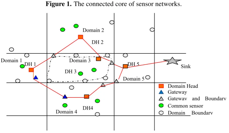
Definition 2 (connected core): Given a graphG = (V, E), the node setCof the graphG = (C⊆V)is a connected core only if C satisfies the following conditions: The subgraph derived fromCis a connected graph, andCis a key node set of graphG. For example, the connected key node set is constructed by the cluster head (with red squares) and the gateway (blue hollow triangle or practice triangle) of the sensor networks in Figure1. The practice triangles in Figure1denote both the gateway and domain boundary sensors (Section 3.3). The practice dots represent the domain-boundary-sensors (Section 3.3), and the green hollow dots are the ordinary sensor nodes.

Figure 1. The connected core of sensor networks. Step 1: Constructing the connected core and dividing the domain of the network by executing ACCC algorithm.

Step 2: determines the initial boundary of heritage site.

Step 3: detects and tracks the deformation of the heritage periodically

3.2 Construction of the Connected Core

3.2.1 Algorithm of Automatic Construction of Connected Core (ACCC)

We assume that all the nodes in the sensor networks can communicate effectively within the same communication range. Two nodes are adjacent if they are within the communication range for each other; actually an adjacent link between two nodes is symmetrical. So, the topology of a sensor network can be a simple connected undirected graph G= (V, E), where V is the set of vertices constituted by all nodes and E is the edge sets of all links. Based on these assumptions, we define the following three concepts as a basis to present our ACCC algorithm.

Definition 1 (Core). Given a graph G = (V, E),where V is the vertices sets of sensor nodes and E is the edge sets of all links, the node set C of G(CV) is a Core if and only if C satisfies that for any node p in V, p either in C or p is a neighbor of the node q in C.

Definition 2 (Connected Core). Given a graph G = (V, E), the node set C of the graph G(CV) is a Connected Core only if C satisfies the following conditions: The sub graph derived from C is a connected graph and C is a key node set of graph G. For example, the connected key node set is constructed by the cluster head (with red squares) and the gateway (blue hollow triangle or practice triangle ) of the sensor networks in Fig.1.The practice triangles in Fig.1 denote both the gateway and domain boundary sensors (section 3.3). The practice dots represent the Domain-Bundary-sensors((section 3.3)and green hollow dot is ordinary sensor nodes.

Definition 3 (Domain). For the random sensor node p, we assume that the coordinate of p relative to the Sink node S is (x, y), Sink node S and all the sensor nodes have the same communication radius r, then p belongs to the domain (m, n) if and only if the following equation holds:

m

=

[

x|

2

r

_],

_n

_{= [}

_y|

2

r

_].

_{Where "/" denote the division operator;}

_{“[ ]”}

_is _{the integer operators for}

taking greater than or equal to an integer.

For example, if r = 15, the geographic coordinates of node A is (40, 40), then Ax=4, Ay=4, so A belongs to the domain (4,4); we assume that the geographic coordinates of B is (51, 53), Bx=5, By=5, so B belongs to the domain(5,5),instead of (4,4).

Domain 4

Domain 1 Domain 3

Domain 5

DH 1 _Sink

Domain Head Gateway

Domain Boundary Common sensor

Gateway and Boundary Domain 2

DH 2

DH 3

DH4

DH 5

(7)

pbelongs to the domain(m, n)if and only if the following equation holds: m = hx/√r

2

i

,n = hy/√r

2

i . Where “/” denotes the division operator; “[]” is the integer operators for taking a valuegreater than or equal to an integer.

For example, if r = 15, the geographic coordinates of Node A are (40, 40); then Ax = 4, Ay = 4.

Therefore,Abelongs to the domain (4,4). We assume that the geographic coordinates ofBare (51, 53), Bx= 5,By = 5, soBbelongs to the domain (5,5), instead of (4,4).

For any sensor node p, we assume that the geographical coordinates are (x, y). All of the nodes, including the sink node S, have the same communication range with a radius ofr. For any sensor node p, we can calculate their respective domain according to Definition 3 and give the following ACCC algorithm. We required that the ACCC must be operated in the connectivity coreCgiven in Definition 3:

Algorithm 2ACCC

Step 1:Every nodepuses the GPS to calculate the geographic coordinates and the remaining energy; calculate the domain according to Definition 3.

Step 2:Every nodepperiodically exchanges the comprehensive state information with its adjacent nodes. Step 3:Set the domain head and/or the domain gateway.

Step 4: When the nodes get the sensing data, the data will be delivered directly to the domain head of the domain.

We explain the ACCC Algorithm 2 as follows. In Step 2, every node p periodically exchanges the comprehensive state information with its adjacent nodes. The comprehensive state information comprises three parameters:

(i) Sp: the current status of node p (every node has three kinds of statuses: domain head, gateway

or ordinary member);

(ii) Ep: the remaining energy ofp;

(iii) Gp: the domain ofp;

(iv) (x,y): the geographical coordinates of p. After this operation, each node can get the adjacent nodes’ information, such as the status of their neighbor nodes, the residual energy, their domain, the straight-line distance to the neighbor node and others.

In Step 3, initially, the status of the sink node is the domain head, while the others are members. In every cycle, node p will calculate its new status according to the following rules by its neighbor’s information, such as the statusSp, the energyEp andGp. If there is no domain head in theGp, the node

with the largest residual energy in theGpwill be selected as the domain head of this domain. Otherwise,

ifpis neither a domain head and gateway nor the neighborhood node of other domain,pis the gateway. In Step 4, when the nodes get the sensing data, the data will be delivered directly to the domain head of the domain.

3.2.2. Connectivity Analysis

(8)

Sensors2014,14 20569

Theorem 1: Assume the sink node S and all sensor nodes in the sensor network have the same communication radiusr; there is the unique division of domain that satisfied the formula in Definition 3.

Theorem 2: Any two sensor nodes in the same domain are adjacent nodes.

Proof: According to Definition 3, the domain is a district of square, and the maximum distance between any two nodes of the region is

r

√

2

+√r

2

=r. Any two nodes are within the radius of each other’s effective communication, so any two sensor nodes in the same domain are adjacent nodes.

As shown in Figure2, letrbe the communication radius of the sensor node; the domain is actually an inscribed square of the circle whose radius isr/2. The distance of any two points in the inscribed square is less thanr, so that all of the nodes within the inscribed square can communicate with each other; thus, any two nodes within an inscribed square are connected.

Figure 2. The inscribed square of the circle.

the adjacent nodes’ information such as the status of their neighbor nodes, the residual energy,

their domain, the straight-line distance to the neighbor node and others.

In step 3, initially, the status of Sink node is the domain head, while the others are member. In every cycle, node p will calculate its new status according to the following rules byits neighbor’s information, such as the status Sp, the energy Ep and the Gp..If there is no domain head in the Gp, the node with the largest residual energy in the Gp will be selected as the domain head of this domain. Otherwise, if p is neither a domain head and gateway nor the neighborhood node of other domain, p is the gateway. In step 4, when the nodes get the sensing data, the data will be delivered directly to the domain head of the domain.

3.2.2 Connectivity Analysis

We can deduce theorem1 and 2 by definition 3:

Theorem1: Assume the Sink node S and all sensor nodes in the sensor network have the same

communication radius r; there is the unique division of domain that satisfied the formula in definition 3.

Theorem 2: Any two sensor nodes in the same domain are adjacent nodes.

Proof: According to definition3: the domain is a district of square, the maximum distance

between any two nodes of the region is 2 2

) 2 ( ) 2

( r  r

=r

. Any two nodes are within the radius of each other's effective communication, so any two sensor nodes in the same domain are adjacent nodes.

As shown in Fig.2, let r be the communication radius of the sensor node, the domain is actually a inscribed square of the circle whose radius is r / 2. For the distance of any two points in the inscribed square is less than r, so all the nodes within the inscribed square can communicate with each other, thus any two nodes within an inscribed square are connected.

Fig 2.the inscribed square of the circle

According to the algorithm ACCC, we know that ACCC is fully distributed.

Theorem 3: Assuming the graph G = (V, E) is a simple connected undirected graph, the

node sets= {p| p is domain head or gateway node and pV} that get from the algorithm ACCC

is a connected Coreof graph G.

Proof:

First of all, we can see from theorem 2 and step 3 of the algorithm ACCC: every node in the set is either a domain head node or its neighbor node is one of domain head at least, namely, it is neighbor with some domain head node. So, the setis a core of the graph G . We proveis connected by induction as follows.

r/2

According to the algorithm ACCC we know that ACCC is fully distributed.

Theorem 3: Assuming the graph G = (V, E) is a simple, connected, undirected graph, the node set ψ ={p |pis the domain head or gateway node andp ∈V}that is obtained from the algorithm ACCC is a connected core of graphG.

Proof: First of all, we can see from Theorem 2 and Step 3 of the algorithm ACCC that every node in the setψ is either a domain head node or its neighbor node is one of the domain heads at least; namely, it is a neighbor with some domain head node. Therefore, the set ψ is a core of the graph G. We prove thatψis connected by induction as follows.

Letpandqbe any two domain head nodes ofψ, that is to say,p,q∈ψ. We have assumed that all of the sensor nodes have the same communication radius, and for convenience of expression, we assume that the communication radius is one unit length; so, the distance betweenpandqis the length of the shortest path betweenpandq, denoted asd(p,q). Since the graph Gis connected,d(p,q)<R(Ris a real number), andd(p,q)is a finite integer.

(1). (i) If d(p,q)= 1, we can deduce that p and q are adjacent, so they are directly reachable. We can deduce thatψ is connected.

(9)

r is the neighbor ofp andq, from Step 3.2 of the ACCC algorithm, ifr is not the domain head, thenrmust be the gateway; therefore,r∈ψ. We can deduce thatψis connected.

(iii) Ifd(p,q)= 3, namely there is a path(p,r1,r2,q)inG. For the reason ofd(p,r2)= 2 ,pandqare

not adjacent, and we know thatpandr2do not belong to the same domain from Theorem 2. From

Step 3.2 of the ACCC algorithm, we know that ifr1 is not a domain head,r1must be the gateway,

andr1is the neighbor ofpandr2; sor1 ∈ψ. For the same reason, sinced(r1,q)= 2, we know that

r2 ∈ψ. We can deduce thatψis connected.

(2). Assume thatψ is connected whend(p,q) =m(m>3).

(3). For d(p,q) = m + 1, there is a path (p,r1,r2,...,rm,q) in G. ψ is the core of graphG, and we can

deduce that r2 is the domain head or r2 are neighbors of a domain head r inψ. We can deduce

d(p,r)≤3. The proof of Step 1 shows that node p and r are reachable in ψ, but d(r,q) ≤ m; the induction assumption shows that node p and r are reachable within ψ. We can deduce ψ is connected.

From Theorem 3, we know that the nodes of setψ build a connected core, and the connected coreψ is constituted of domain head nodes and gateway nodes. The Skyline query message and resulting data can be forwarded along the nodes inψ. Compared to the entire network, the number of nodes in theψ is much less, which can dramatically reduce network traffic.

3.3. Boundary Detection and Tracking

The key point for detection and tracking of deformation is to construct a set of connected core nodes in the sensor networks during the initial phase. As shown in Figure 1, one node within each domain is nominated as the head and plays the role of a local controller. The normal nodes get the sensor data of the environment and send or relay the sensing data to the domain head (DH). The DH generates sensing data of its own, collects the data sent from the normal nodes in the domain and fuses and transfers this information to the sink via the connected core path.

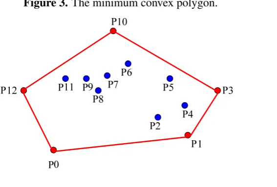
When the DH receives the location information from all of the normal nodes in the domain, the DH detects the sensors located around at the boundary of the heritage object and notifies them that they are the boundary sensors of the heritage object. The boundary sensors are selected from the normal nodes in a domain through finding the minimum convex polygon that contains the heritage object. For a subset S ofn-dimensional spaceR,t convex MCP(K) is defined as the smallest convex set in R. For example, the convex polygon represented by the red line shown in Figure 3is the minimum convex polygon of convex setQ = {p0,p1...p12}. We present the algorithm for finding boundary sensors in Section3.3.1; the

method for finding the minimum convex polygon in geometry refers to [35]. 3.3.1. Finding Boundary Sensors (FBS) Algorithm

(10)

Sensors2014,14 20571

Figure 3. The minimum convex polygon.

Fig 3. The minimum convex polygon

3.3.1. Finding the boundary sensors (FBS) algorithm

Let all the nodes in a domain represent the subset S of n dimensional space R, and the DH distinguishes the boundary sensors among them by using thefinding the boundary sensors (FBS) algorithm as follows.

Definition 4, rotation direction of the path: Let o=(xo,yo), p=(xp,yp), q=(xq,yq) are any three

nodes in the domain, vector D(o,p,q)denote the rotation direction of the path.

1 ( , , )

1

o o

p p o o p q q o o p p o q o

q q

x y

D o p q

x y

y x

x y







If D>0,then the path o,p,q,o form an anti-clockwise loop; if D<0, then the path o,p,q,o form form a clockwise loop; if D=0, o, p, q are collinear.

We first identify the smallest y coordinate of nodes in S, assumed p0, and establish a coordinate

axis whose origin is p0, (if two nodes pi and pj have the same smallest y coordinate and pi.x< pj.x,

we select pj as its origin). The other nodes are mapped to the p0 origin coordinate axis system.

After mapping all the nodes into the p0 origin coordinate axis system, we compute all the node’s

slope and sort all the nodes in ascending order according node’s slope, and get the sorted nodes set T={p1,p2,….Pn},where p1and Pn have the smallest and largest slope respectively.

Second, we establish the stack ST(S), which is initialized to ST(S) = {Pn, p0}. Without loss of

generality, We aassume that at a time the ST(S)={ Pn, p0…pi,pj,pk},where pk is on the top of ST,

and the nodes in ST have constituted a semi-closed convex polygon(Fig 4.a), pl is the next node in

the T. If the rotation direction D(pj,pk,pl) >0, then the path pj, pk, pl form an anti-clockwise loop

and pj, pk, pl will form a convex polygon, and thepk, pl will be a convex polygon edge. We pushpl

into stack ST(S). if D(pj,pk,pl) >0, then the path pj, pk, pl form an clockwise loop and the pk, pl will

not be a convex polygon edge. We pop pk out of stack ST(S).（Fig.4.b and Fig.4.c）. Finally, the

nodes in ST are the boundary sensors which determine the boundaries of heritage.

Algorithm 3Finding the boundary sensors (FBS) algorithm 1: Input a set of sensorsS = {p0,p2,...Pn−1}.

2: Select the rightmost and lowest sensorp0 as the original and establish a coordinate axis whose origin isp0.

3: Map the other sensorSinto thep0origin coordinate axis system.

4: Compute the slope of the sensorS.

5: LetT[n]be the sorted arraySin ascending order.

6: PushT[n−1]andp0 onto a stackST, andspdenotes the stack point ofST.

7: WHILE i<n.

8: IFD(ST[sp],ST[sp−1],T[i])≥0,THEN 9: PushT[i]intoST

10: i++ 11: ELSE

12: pop theD(ST[sp]off theST. 13: sp = sp-1.

14: ENDIF

15: ENDWHILE 16: Output:ST.

Definition 4, Rotation direction of the path: Let o = (xo,yo), p = (xp,yp), q = (xq,yq) are any three

nodes in the domain, vectorD(o,p,q)denotes the rotation direction of the path.

D(o, p, q) =

xo yo 1

xp yp 1

xq yq 1

=xoyp+yoxq+xpyp−xqyp−yqxo−xpyo

If D> 0, then the path <o,p,q,o> forms an anti-clockwise loop; ifD < 0, then the path (o,p,q,o) forms a clockwise loop; ifD = 0, o, p, qare collinear.

We first identify the smallesty coordinate of nodes inS, assume p0 and establish a coordinate axis

whose origin isp0(if two nodespiandpjhave the same smallestycoordinate andpi.x<pj.x, we selectpj

as its origin). The other nodes are mapped to thep0origin coordinate axis system. After mapping all of

(11)

nodes in ascending order according to the node’s slope and get the sorted nodes setT = {p1,p2,â ˘A˛e.pn},

wherep1andPnhave the smallest and largest slope, respectively.

Second, we establish the stack ST(S), which is initialized to ST(S) = {Pn, p0}. Without loss of

generality, We assume that at a time, the ST(S) = {Pn, p0...pi,pj,pk}, where pk is on the top of ST,

and the nodes in ST have constituted a semi-closed convex polygon (Figure 4a); pl is the next node

in theT.

If the rotation directionD (pj,pk,pl)>0, then we pushplinto stackST(S), since the path<pj,pk,pl>

forms an anti-clockwise loop and <pj, pk, pl> forms a convex polygon, and the pk, pl are a convex

polygon edge. If D (pj,pk,pl) >0, then we pop pk out of stack ST(S) (Figure 4b,c), since the path

<pj,pk,pl>forms an clockwise loop andpk,plare not a convex polygon edge. Finally, the nodes inST

are the boundary sensors that determine the boundaries of a heritage object.

Figure 4. Finding the boundary sensors.

Fig.4 finding the boundary sensors

Table 3. Finding the boundary sensors (FBS) algorithm

Algorithm: Finding the boundary sensors

1:Input a set of sensors

S

=

{

p

0

,p

2

,….P

n-1

}

2:Seletct the rightmost and lowest sensor

p

0

as the original, and establish a coordinate axis

whose origin is

p

0

.

3: map the other sensor s into the

p

0

origin coordinate axis system.

4:compute the slope of the sensor s

4: let

T[n]

be the sorted array

S

in ascending order.

5:push

T[n-1]

and

p

0

onto a stack

ST

, and

sp

denote the stack point of

ST

.

6:

WHILE

i<n

7:

IF

D(

ST[sp]

,

ST[sp-1],T[i]

)



0 THEN

8: push

T[i]

into

ST

9: i++

10:

ELSE

11: pop the

ST[sp]

off the

ST

12 ：

sp

=

sp

-1

13:

ENDIF

14:

ENDWHILE

15:output:

ST

3.3.2. Boundary detection

This subsection describes the use of the FBS presented above to perform the boundary

detection of a heritage site.

Firstly, the DH finds the boundary of the domain. The DH determines those sensors residing at

(a)

Fig.4 finding the boundary sensors

Table 3. Finding the boundary sensors (FBS) algorithm

Algorithm: Finding the boundary sensors

1:Input a set of sensors

S

=

{

p

0

,p

2

,….P

n-1

}

2:Seletct the rightmost and lowest sensor

p

0

as the original, and establish a coordinate axis

whose origin is

p

0

.

3: map the other sensor s into the

p

0

origin coordinate axis system.

4:compute the slope of the sensor s

4: let

T[n]

be the sorted array

S

in ascending order.

5:push

T[n-1]

and

p

0

onto a stack

ST

, and

sp

denote the stack point of

ST

.

6:

WHILE

i<n

7:

IF

D(

ST[sp]

,

ST[sp-1],T[i]

)



0 THEN

8: push

T[i]

into

ST

9: i++

10:

ELSE

11: pop the

ST[sp]

off the

ST

12 ：

sp

=

sp

-1

13:

ENDIF

14:

ENDWHILE

15:output:

ST

3.3.2. Boundary detection

This subsection describes the use of the FBS presented above to perform the boundary

detection of a heritage site.

Firstly, the DH finds the boundary of the domain. The DH determines those sensors residing at

(b)

Fig.4 finding the boundary sensors

Table 3. Finding the boundary sensors (FBS) algorithm

Algorithm: Finding the boundary sensors

1:Input a set of sensors

S

=

{

p

0

,p

2

,….P

n-1

}

2:Seletct the rightmost and lowest sensor

p

0

as the original, and establish a coordinate axis

whose origin is

p

0

.

3: map the other sensor s into the

p

0

origin coordinate axis system.

4:compute the slope of the sensor s

4: let

T[n]

be the sorted array

S

in ascending order.

5:push

T[n-1]

and

p

0

onto a stack

ST

, and

sp

denote the stack point of

ST

.

6:

WHILE

i<n

7:

IF

D(

ST[sp]

,

ST[sp-1],T[i]

)



0 THEN

8: push

T[i]

into

ST

9: i++

10:

ELSE

11: pop the

ST[sp]

off the

ST

12 ：

sp

=

sp

-1

13:

ENDIF

14:

ENDWHILE

15:output:

ST

3.3.2. Boundary detection

This subsection describes the use of the FBS presented above to perform the boundary

detection of a heritage site.

Firstly, the DH finds the boundary of the domain. The DH determines those sensors residing at

(c)

3.3.2. Boundary Detection

Heritage Object Deformation Detecting by Checking the RSSI of Anchor Nodes

The wireless signal energy will decay with increasing distance in the process of communication. The signal energy received by the node is the RSSI. According to the log path loss model in [36], the received signal energy decay in a logarithmic trend with distance increases. If both the transmission energy and the received signal energy can be obtained at the receiving end, the signal attenuation can be obtained according to Formula (1) as follows:

Pr(d)[dBm] =P0(d0)−10nlog10(

d d0

) (1)

where d0 is the reference range, P0(d0) and Pr(d) are the received signal strength in d0 and d,

respectively, andnis the path loss exponent. We know from Formula (1) that the received signal strength of nodes is a function of the distancedand will be changed with the variation ofd.

Transform Formula (1) to Formula (2):

d=10p0(d0)[dBm10]−npr(d)[dBm]

(12)

Sensors2014,14 20573

According to Formula (2), givenPr(d), d0 andP0(d0), we can get the new reference ranged, where

the path loss exponent n is a fixed value and can be measured in an experiment if the environment is unchanged.

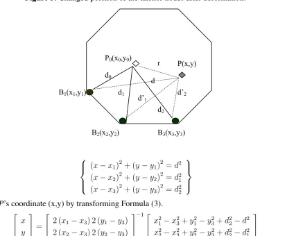
For example, In Figure 5, The new position of anchor node P0 is P, the distance betweenPand

B1, B2, B3 is d, d1, d2, respectively, and the coordinate of B1, B2, B3 is (x1, y1)ïij ˇN(x2, y2),(x3, y3),

respectively. We can get the new position of P’s coordinate (x,y) according to Formula (3). By fusing the RSSI data of anchor nodes that are deployed on the heritage object, we can accurately calculate the heritage deformation size and angle. According to our actual experiment, the average positioning error is 0.115 m.

Figure 5. Changed position of the anchor nodes after deformation.

Fig.5 Changes position of anchor nodes after deformation

Transform the formula (1) to formula (2):

0( 0)[ ] ( )[ } 10

0

10

r p d dBm p d dBm

n

d









_

_







(2)

According to formula (2), given

P d

_r

( )

,

d

₀ and

P d

₀

( )

₀ ,we can get the new

reference range d , where the path loss exponent n is a fixed value and can be measured

in experiment if the environment unchanged.

For example, In Fig5, The new position of anchor node P0 is P, the distance

between P and B1,B2,B3 is d,d1,d2 respectively, and the coordinate of B1,B2,B3 is (x1,y1)， (x2,y2),(x3,y3) respectively. We can get the new position of P’s coordinate (x,y) according to formula (3). By fusing the RSSI data of anchor nodes which deployed on the heritage, we can accurately calculate the heritage deformation size and angle. According to our actual experiment, the average positioning error is 0.115 meters.

2 2 2

1 1

2 2 2

2 2 1

2 2 2

3 3 2

(

)

(

)

(

)

(

)

(

)

(

)

x

y

d

x

y

d

x

y

d

 







 









 









（3）

We get the P’s coordinate (x,y) by transform the formula (3).

B1(x1,y1)

P0(x0,y0)

P(x,y)

B2(x2,y2) B3(x3,y3)

d0

d1

d2

d’1

d’2

d r

  

 

(x−x1)2+ (y−y1)2 =d2 (x−x2)2+ (y−y2)2 =d21 (x−x3)

2

+ (y−y3) 2

=d2 2

  

 

(3)

We getP’s coordinate (x,y) by transforming Formula (3). "

x y

#

=

"

2 (x1−x3) 2 (y1−y3) 2 (x2−x3) 2 (y2−y3)

#−1" x2

1−x23+y21 −y32+d22−d2

x2

2−x23+y22 −y32+d22−d21

#

In the actual environment, the signal attenuation model is influenced by the influencing factors, such as temperature, humidity, wind and other environmental factors, such as voltage and antenna. The signal attenuation model is not an ideal type as Formula (1), but in line with the normal distribution related to the distance [36], as shown in Formula (4).

Pr(d) [dBm] =P0(d0)−10nlog10

d d0

+Xσ (4)

whereXσ is the random variable in line with the normal distribution;σis the noise factor under specific

circumstances. When the environment is stable, the path loss exponent n and noise factor σ can be considered as a fixed value and can be obtained in an experiment. Therefore, Pr(d)is a function of d

(13)

replaceP0(d)andPr(d)withE(P0(d))andE(Pr(d)), as well as replaceXσ withX¯σ, whereE(P0(d))is

the expected value of the received signal strength ofP0(d),E(Pr(d))is the expected value of the received

signal strengthPr(d),X¯σ is the mean value ofXσ. We can get Formula (5) from Formula (2).

d=10E(p0(d0)[dBm])−10En(pr(d)[dBm])+ ¯Xσ

×d0 (5)

Heritage Object Deformation Detecting by Boundary Detection of Heritage Site

Firstly, the DH finds the boundary of the domain. The DH (domain head) determines the sensors located at the boundary of the domain and notifies them to be the boundary sensors of the domain. The DH determines the boundary sensors among the normal nodes in the domain by the FBS algorithm in Algorithm3. Note that hereafter, the boundary sensors of the domain are referred to as domain-boundary sensors (DBs), while the remaining nodes are referred to as normal sensors (Ns). As show in Figure1, the shaded gray nodes represent the DBs of the corresponding domain.

The control messages are used to transmit the detecting information to the DH whenever the object is detected. There are “Detecting” and “Domain” in the control message. The format of “Detecting” and “Domain” is number. The “Detecting” implicate the Domain-boundary-sensors detect the target heritage, while “Domain” is the number of domain where the heritage is detected.

“Detecting”: is used only by the DBs and is sent to the DH once the DBs detect the target heritage. For example, when the DBs detect the collapse of the large heritage and parts of the heritage move into the domain, The DBs will set the “Detecting” to ‘1’ and send to DH.

“Domain”: is used only by the Ns. It is set to ‘n’ when the detected heritage is identified within domainn.

When the collapse or the deformation of the heritage object is detected, a DBs communicates with all of the one-hop neighboring DBs in other domains to query their detection information. Once the DBs has received this information, it sets “domain” to ‘n’ in the control message and sends it to the DH, such that the DH can determine all of the domains within which the heritage has spread. For example, we consider a network system comprised of just five domains, as shown in Figure 6. Two particular scenarios are presented in the following to explain how many domains the heritage object covers.

Scenario 1: Within a Single Domain or Covers the Whole Domain

(14)

Sensors2014,14 20575

Sand applies the FBS to get the corresponding boundary sensor set of the heritage object; for example, the boundary sensor set indicated by the dotted line in Figure6a.

Figure 6. Boundary detecting and tracking of a heritage object. (a) The heritage object covers a single domain; (b) the heritage object shape fully covers a domain; (c) the heritage shape spread across two domains; (d) the heritage shape spread across three domains.

(a) (b)

(c) (d)

Fig.5 Boundary detecting and tracking of heritage: (a)heritage shape lies within a single domain;(b) heritage shape fully covers a domain;(c) heritage shape spread across two domains;(d) heritage shape spread across three domains.

1. Within a single domain or Covers the whole domain

The scenario in Fig. 5(a) shows that the heritage (indicated by the solid curve) is located entirely within a single domain (domain3). In this case, after sensing the heritage, the Ns within

the object boundary broadcast‘Detecting’ messages to notify DH3 that they have detected the

heritage. Meanwhile, when the DBs in Dmain3 (i.e., Sensors A, B, C) detect the heritage, they query the object detection information of their one-hop neighboring DBs in domain 4 and 5 and determine that the detected heritage does not extend beyond the boundary of domain 3. the DBs set the ‘3’ to ‘Domain’ in the control message and sent it to DH3. When receiving these messages, DH3 determines that the detected object is currently spread only within its own domain DH3. Use FBS to distinguish the boundary sensors of the heritage, treats all of the sensors (including both

Common sensor Domain Head Domain Boundary DH 5

Domain1 Domain 3 DH 2 Domain 2

A B C

DH 1

Domain 4

Domain 5

DH 3 DH4

Domain 5 G F E C B A Common sensor Domain Head Domain Boundary Domain 1 DH1 Domain4 Domain3 Domain2DH2 DH3 DH4 DH5 DH 1 Common sensor Domain Head Domain Boundary Domain 5

Domain 1 Domain 3 Domain 4

Domain 2 DH 2

DH 3

DH4

DH 5

E F G

D

A B C

C A

Domain 3

E F G

Common sensor Domain Head Domain Boundary DH 2 Domain 5 Domain 1 DH 1 Domain 4 Domain2 DH4 DH 5 B DH3 D (a)

(a) (b)

(c) (d)

A B C

DH 1

Domain 4

Domain 5

DH 3 DH4

Domain 2 DH 2

DH 3

DH4

DH 5

E F G

D

A B C

C A

Domain 3

E F G

Common sensor Domain Head Domain Boundary DH 2 Domain 5 Domain 1 DH 1 Domain 4 Domain2 DH4 DH 5 B DH3 D (b)

(a) (b)

(c) (d)

A B C

DH 1

Domain 4

Domain 5

DH 3 DH4

Domain 2 DH 2

DH 3

DH4

DH 5

E F G

D

A B C

C A

Domain 3

E F G

Common sensor Domain Head Domain Boundary DH 2 Domain 5 Domain 1 DH 1 Domain 4 Domain2 DH4 DH 5 B DH3 D (c)

(a) (b)

(c) (d)

A B C

DH 1

Domain 4

Domain 5

DH 3 DH4

Domain 2 DH 2

DH 3

DH4

DH 5

E F G

D

A B C

C A

Domain 3

E F G

Common sensor Domain Head Domain Boundary DH 2 Domain 5 Domain 1 DH 1 Domain 4 Domain2 DH4 DH 5 B DH3 D (d)

(15)

Scenario 2: Crosses Multiple Domains

Figure 6c,d illustrates the scenario in which the heritage extends across two and three domains respectively; for the scenario in Figure6c, the Ns in Domain 3 transmit “detecting” messages to DH3, as long as they detect the whole or parts of the heritage. Meanwhile, DBs A, B, and C query their one-hop neighboring DBs,i.e., E, F and G, respectively; these sensors report that the object has indeed spread to Domain 5, and thus, DBs A, B and C set ‘3’ and ‘5’ to “domain” in the control message and then send it to DH3 (note that DBs D queries its neighbor in Domain 4). When DH3 receives the control messages, it learns that the detected heritage object is not confined solely within its own domain, but has also spread to Domain 5. As for the scenario in Figure 6d, DH3 learns that the detected heritage object is spread across three domains. If the heritage object crosses multiple domains, the domain head will estimate the portion of the boundary lying within its own domain, fuses the boundary information in a compact data format and then relays it to the sink via the connected core. The sink determines the entire boundary of the heritage site by compiling the integrated boundary information received from all of the domain heads in the network. The heritage object boundary detection (HBD) algorithm is presented in Algorithm 4.

Algorithm 4Heritage boundary detection (HBD) algorithm 1: IFthe heritage within a single domain,THEN

2: get the heritage object boundary by executing FBS. 3: ELSE

4: DHs estimates the portion of the object boundary lying within its own domain by executing the BPE (the boundary portion estimation algorithm (Algorithm5)).

5: All DHs fuse the boundary information in a compact data format and then relay it to the sink.

6: The sink determines the entire boundary of the heritage by compiling the integrated boundary information received from all of the DHs in the network.

7: ENDIF

Algorithm 5The boundary portion estimation algorithm (BPE)

Step 1: DHs distinguish the domain boundary sensors among all of the sensors that have detected the heritage object by FBS.

Step 2:DHs identify and eliminate the redundant sensors in the domain boundary set. Step 3:DHs eliminate any non-boundary sensor(s) from the heritage object boundary set.

In Step 2, the DH identifies and eliminates the redundant sensors in the domain boundary set by eliminating the DBs that separate the distance into two sensor pairs. For example, in Figure 6c, DH3 calculates the straight line distance between each pair of DBs along the common border between Domains 3 and 5, which have detected the heritage object, i.e., A and B, B and C and A and C; the distance between A and C is greater than that between A and B or B and C, respectively, and thus, B is eliminated. In Figure6d, DH3 removes the redundant sensors, B and D.

(16)

Sensors2014,14 20577

a domain-boundary sensor in Domain 3, but also has the information that the shape of the detected heritage object spreads across more than two domains. Therefore, DH3 further eliminates NodeCfrom the heritage object boundary set.

3.3.3. Boundary Tracking and Deformation Detection Boundary Tracking

After being deployed and initialized, EffeHDDT operates in the monitoring phase; the EffeHDDT method detects the heritage object boundary periodically. When a portion of or the whole heritage object boundary moves out of the sensing range of the current boundary sensors (for example, the deformation and collapse of the heritage object), on receiving these messages and examining the “domain” information they contain, DH identifies the nodes within its domain that represent the new boundary sensors of the heritage object by executing the heritage object boundary detection algorithm (Section 3.3.2), and the heritage object boundary node set must be updated to be responsible for the new boundary location. If a sensor detects the disappearance of the heritage object in its local area at the current time slot, it knows that the boundary of the heritage object moved through its detection area during the past time slot. In such a situation, the sensor set the “detection” to ‘−1’ in the control message to notify its DH of updating the heritage object boundary information.

Figure7illustrates a change in the position of the object boundary and the subsequent changes in the boundary profile portions in Domains 3, 4 and 5, respectively. Note that in these figures, the region via the thick dotted line represents the location of the heritage object in the previous time slot, and the circles connected via the thin dotted lines represent the old boundary sensors. Meanwhile, the curve marked using a thick solid line represents the new boundary. In the current time slot, the Ns and DBs in each domain sense the heritage object for the first time and send “detecting” and “domain” messages to their DH, and the EffeHDDT method identifies the new boundary sensors of the heritage object by executing the heritage object boundary detection algorithm (Section 3.3.2). The circles connected via red dashed lines in each static domain in Figure7indicate the new boundary sensors of the object, as determined by DHs 3, 4 and 5, respectively.

Figure 7. Updating boundary sensors when a heritage object is deformed or has a moving boundary.

Table 5. the boundary portion estimation algorithm

Algorithm: the boundary portion estimation algorithm

Step 1: DHs distinguish the domain boundary sensors among all of the sensors which have detected the heritage by FBS.

Step 2: DHs identify and eliminate the redundant sensors in domain boundary set.

Step3: DHs eliminate any non-boundary sensor(s) from the heritage boundary set.

In step2, DH identify and eliminate the redundant sensors in domain boundary set by eliminating the DBs that separate the distance into two sensor pairs. For example, in Fig.5(c), DH3 calculates the straight line distance between each pair of DBs along the common border between Domain 3 and 5which have detected the heritage, i.e., A and B, B and C, and A and C, the distance between A and C is greater than that between A and B or B and C, respectively, and thus B is eliminated. In the Fig.5(d), DH3 remove the redundant sensors B and D.

In step 3, on the base of step2, DHs eliminate the redundant sensors which have the

information that the shape of the detected heritage spreads across multiple Domains. For example in Fig.5(d), it is easily determined that C cannot be a boundary sensor of the heritage since it is not only a Domain-boundary sensor in Domain3, but also has the information that the shape of the detected heritage spreads across more than two domains. Therefore, DH3 further eliminates C from the heritage boundary set.

3.3.4 Boundary Tracking and Deformation Detection

1 、

Boundary Tracking

Fig.6 updating boundary sensors when heritage deformed or moving boundary

After deployed and initialed, the EffeHDDT operates in the monitoring phase, the EffeHDDT detects the heritage boundary periodically. When a portion of or the whole heritage boundary

DH 3

Common sensor Domain Head Domain Boundary Domain 1

E

A B C

F G

Domain 3 DH 2

Domain 5

Domain 4 Domain 2

DH4

DH 5

(17)

Deformation Detection

EffeHDDT detects the deformation of heritage object by the heritage object boundary similarity mechanism. The main idea is to save the latest heritage object boundary information OCP (old convex polygon) calculated in the last round in the DH or sink. In the new period, EffeHDDT will get the new heritage object boundary information NCP (new convex polygon), then calculate the similarity of the OCP and NCP (SM (C) Similarity). The heritage object deformed only when SM (C) is less than the threshold K(SM(C) < K) (in this paper, K = 0.93, 0.93 is given by the heritage experts [2]). At the same time, EffeHDDT broadcasts the threshold K to DHs and boundary nodes. DH and boundary nodes calculated the similarity and forwarded the new boundary information only when the similarity was less thanK.

How does one calculate the convex polygon similarity? The two convex polygons are similar if they are topologically similar, geometrically similar, directionally similar and have the same area; the two convex polygons are topologically similar if they have a one to one corresponding relationship in the geometry element type and connection sequence; the two convex polygons are geometrically similar only if they are topologically similar and their connected type (vertical, tangent connection,etc.) of geometry element has a one to one corresponding relationship; the two convex polygons are directionally similar if they have the same angle between the minimum polygon rectangle and the horizontal axis; the two convex polygons are similar if they are topologically similar, geometrically similar, directionally similar and have the same area. The convex polygon similarity SM (C) can be defined as:

SM(C) =K1×sm(T op log y) +K2×sm(Geometry) +K3×sm(Direction) +K4×sm(Area) (6)

wheresm(Top log y), sm(Geometry), sm(Direction)andsm(Area)are the topology similarity, geometry similarity, direction similarity and area similarity of the convex polygon, respectively. K1, K2, K3, K4

are the weight andK1+K2+K3+K4= 1. Similar to the image similarity calculation [37], we give the

following general formula ofsm(T),

sm(T) = M

P

i=1 N

P

j=1

αijβij

M ×N (7)

where αij is the geometric elements of convex polygons and βij is a similar coefficient of geometric

elements [37].

4. Performance Evaluation

In this Section, we demonstrate the effectiveness and efficiency of EffeHDDT by a real node experiment and a simulation experiment.

4.1. Real Node Experiment

(18)

Sensors2014,14 20579

to maintain the indoor temperature, to keep wind and dust stable and to maintain dryness, and at the same time, there is special equipment to screen out strong electric and magnetic fields.

In the experiment, we use the MICAz node of Crossbow to collect the RSSI value and to create a sample database. Ten anchor nodes are deployed randomly in the 10 m × 10-m region, which is surrounded by 30 boundary nodes. The average of the three boundary nodes corresponds to one anchor node to calculate the RSSI value. In order to simulate random heritage object deformation, we move the position of the anchor node randomly. The distance of each movement is limited to 0.2 m, and it must be ensure that the anchor nodes cannot move out of the scope of the boundary nodes. We collect 1000 data at each distance; 60% of them are treated as the sample data for training, and the remaining 40% are treated as test data; the abnormal data are processed before the training samples.

The average weighted distance is calculated following Formula (6) acting as the estimation distance between boundary nodes and anchor nodes. We define distance error as follows: distance error = actual distance−estimation distance. The actual distance is the line measuring the distance between boundary nodes and anchor nodes.

Figure8shows that the distance error results of EffeHDDT fluctuates between 0.015 to 0.025, which is a reasonable error range for a site deformation decision [2].

Figure 8. The distance error of EffeHDDT.

training samples.

The average weighted distance is calculated following formula (6) acted as estimation distance between boundary nodes and anchor nodes. We define distance error as follow: distance error= actual distance- estimation distance. Figure 78 shows the distanceerrorresults of EffeHDDTfluctuates between0.015to 0.025, which is areasonable error range forsite deformation decision [29]

EffeHDDT

0 0.005 0.01 0.015 0.02 0.025 0.03

1 3 5 7 9 11 13 15 17 19

The Actual Distance*0.2(m)

T

he

Di

st

an

ce

E

rr

or(

m)

EffeHDDT

Fig.7 The distance error of EffeHDDT

We carry out a positioning error experiment to test the positioning accuracy of EffeHDDT. If anchor node P’s coordinates in the Pi position is (xi, yi) and was moved by K times, the final estimated position coordinate is (xi’, yi’). The definition of positioning error



for the anchor node is:

' '

1

(

) (

)

(

)

2

k

i i i i

i

x

y

k













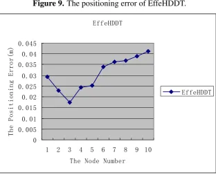
(8)

Figure 8 shows the positioning error results of EffeHDDTfluctuates between 0.018to 0.042, which is areasonable error range forsite deformation decision [29]

We carry out a positioning error experiment to test the positioning accuracy of EffeHDDT in the same experiment environment as the distance estimation experiment. If anchor nodeP’s coordinates in the Pi position is (xi, yi)and was moved byK times, the final estimated position coordinate is(x

0

i, y

0

i).

The definition of positioning errorγ for the anchor node is:

γ = k

P

i=1

_p

(xi−x

0

i)2+ (yi −y

0

i)2

k (8)

(19)

Figure 9. The positioning error of EffeHDDT.

EffeHDDT

0 0.005 0.01 0.015 0.02 0.025 0.03 0.035 0.04 0.045

1 2 3 4 5 6 7 8 9 10

The Node Number

Th

e

Po

si

tio

ni

ng

E

rr

or

(m

)

EffeHDDT

Fig.8 The positioning error of EffeHDDT

4.2. Simulation experiment

using two metrics: the average communication cost and precision of the detection bourndary. Also, wWe analyze the time efficiency of EffeHDDT by recording the average processing time for

issuing a query to the network to obtain all the results. All the simulation experiments run in the

network simulator 2 (ns2) [19].

We assume that the sensor network is randomly deployed in a simulated 1000m x 1000m sensing field. The radio range of each sensor was assumed to be 3m. Two heritage sits/objects are simulated to be detected and tracked within the sensing field, a rectangle with 200m x 100m and a circle with a radius of 100m respectively. We assume that the rectangular and circular objects are initially centered at coordinates of (500, 600) and (200, 200) respectively. The sink is located at coordinates (0, 0). In order to simulate the deformation and collapse of the heritage, the width and length of the rectangular heritage and the radius of the circular heritage increase by 0.1 m in each

time slot, and the system generates a tension value V randomly at same time, when the surface

pressure exceeds V, the heritage object is split into multiple small parts and move around with a

random speed.

4.2.1 Communication cost

In this section, we analyze the communication costs incurred in detecting and tracking the boundary deformation and collapse of the heritage. The communication cost is defined as the total

number of messagesdata packets broadcast in establishing the boundary nodes, integrating the

local boundary information and then disseminating this information to the sink. In the simulations of the message cost, the sensing field is assumed to contain a total of 2500 sensors.

We compare the communication cost of our EffeHDDT method with those of both CODA and

DCS in three different boundary sizes in Fig. 9 and Fig.10. We first introduce the simulation setup.

In Fig.7 (a)-(c), we adopt a maximum number of 80, 160, and 220 boundary sensors with dynamic

clusters in DCS, and 50 static and 50 domains in both CODA and EffeHDDT. In Fig.89(a)-(c), we

adopt 50,100,150 dynamic clusters without limitation of size in each dynamic cluster in DCS, and 50 static clusters and 50 domains in both CODA and EffeHDDT. Then, comparing the three

schemes, the overall trend in both Fig. 7 9 and Fig. 8 10 is that EffeHDDT results in a

considerably lower communication overhead, since EffeHDDT constructs the connected core and

4.2. Simulation Experiment

We analyze the time efficiency of EffeHDDT by recording the average processing time for issuing a query to the network to obtain all of the results. All of the simulation experiments run in the network simulator 2 (ns2) [38].

We assume that the sensor network is randomly deployed in a simulated 1000 m×1000-m sensing field. The radio range of each sensor was assumed to be 3 m. Two heritage sits/objects are simulated to be detected and tracked within the sensing field, a rectangle of 200 m ×100 m and a circle with a radius of 100 m, respectively. We assume that the rectangular and circular objects are initially centered at coordinates of (500, 600) and (200, 200), respectively. The sink is located at coordinates (0, 0). In order to simulate the deformation and collapse of the heritage object, the width and length of the rectangular heritage object and the radius of the circular heritage object increase by 0.1 m in each time slot, and the system generates a tension valueVrandomly at the same time, when the surface pressure exceedsV, the heritage object is split into multiple small parts and moves around with a random speed.

4.2.1. Communication Cost