P-OMP-IR Algorithm for Hybrid Precoding in Millimeter Wave MIMO Systems

P-OMP-IR Algorithm for Hybrid Precoding in Millimeter Wave

MIMO Systems

Ruiyan Du1, Fulai Liu1, *, Xinwei Wang2, Qingping Zhou3, and Xiaoyu Bai2

Abstract—This paper presents a P-OMP-IR algorithm for the hybrid precoding problem in millimeter wave (mm-Wave) multiple-input multiple-output (MIMO) systems. In the proposed approach, the digital precoding matrix is updated via the orthogonal matching pursuit (OMP) method, and the analog precoding matrix is refined column by column using the dominant singular value and corresponding singular vectors of a residual matrix successively. During the refining phase of the analog precoding matrix, an extended power method is designed to calculate the dominant singular value and the corresponding left and right singular vectors, which is able to reduce the computational complexity significantly. Simulation results show that the proposed algorithm can not only reduce the residual of the hybrid precoder effectively, but also improve the spectral efficiency consistently.

1. INTRODUCTION

Millimeter wave (mm-Wave) multiple-input multiple-output (MIMO) system is emerging as a promising technology for the next generation communication [1]. Although mm-Wave MIMO systems experience higher path loss than existing cellular systems, they can take advantage of the large bandwidth in mm-Wave spectrum and employ large-scale antenna arrays that are packed in a very small area due to short wavelength. With large number of antenna elements at the transmitter/receiver, mm-Wave MIMO array can provide significant beamforming gains to combat path loss [2].

Hybrid precoding architecture has attracted wide attention recently, which only requires a small number of radio frequency (RF) chains between the low-dimensional digital precoder and high-dimensional analog precoder [3]. Several methods of hybrid precoder are conceived in [4–6], including the optimal analog beamforming of clustered subarrays [4], minimum-mean-square-error (MMSE)-based analog/digital beamforming [5], and joint transmit/receive beamforming [6]. The convex quadratic programming method and least squares method are utilized to obtain the analog precoding matrix and digital precoding matrix in [7]. A restricted set of dominant candidate directions is leveraged to find the analog precoding matrix in [8]. A successive interference cancelation-based hybrid precoding scheme for subarray structures is proposed in [9]. The advantages of directional beamforming are studied by considering two-path mm-Wave channels in [10]. In [11, 12], the hybrid precoding problem is reformulated as a sparse signal reconstruction problem and solved via the orthogonal matching pursuit (OMP) method. The sparse hybrid precoding algorithm can approach the full digital MIMO processor by iteratively selecting a beamforming vector from the set of array response vectors; however, due to the limited size of the set of array response vectors, the sparse hybrid precoding algorithm still inevitably leads to performance losses.

In this paper, a P-OMP-IR algorithm is proposed to further improve the performance of the sparse hybrid precoding. The hybrid precoding matrix of the proposed algorithm is initialized through the OMP algorithm. Then, each column vector of the analog precoding matrix is refined by using the

Received 10 April 2018, Accepted 9 May 2018, Scheduled 16 May 2018

* Corresponding author: Fulai Liu ([email protected]).

dominant singular vectors of a residual matrix. Afterwards, with the refined analog precoding matrix, the digital precoding matrix is updated via the OMP method again. Finally, by alternatively iterating the above stages, the performance of the hybrid precoder is improved gradually. It is noteworthy that the proposed algorithm depends on the dominant singular vectors of a residual matrix. In order to reduce the computational complexity, an extended power method is proposed to derive the dominant left and right singular vectors simultaneously.

The remaining part of this paper is organized as follows. The system model is introduced in Section 2. Section 3 presents details of the proposed algorithm. Simulations are given to demonstrate the performance of the proposed method in Section 4. Section 5 concludes the paper.

Notations: A stands for a matrix. a represents a vector. A(_m,n) denotes the element of A corresponding to the mth row and nth column. A(:_,n) represents the nth column of A. A(:,1:n) is the first n columns of A. A(_n,:) represents the nth row of A. (A)T, (A)H, (A)−1 and (A)† denote the transpose, the conjugate transpose, the inverse and the pseudoinverse of A, respectively. I_N is the

N ×N identity matrix. |A|,A2 andAF represent the determinant, the 2-norm and the Frobenius

norm of A, respectively. CN(a, b) is a complex Gaussian distribution with mean a and variance b. diag(A) is a vector which consists of the diagonal elements ofA. diag{a1,· · · , aN}is a diagonal matrix

with the entries in{a1,· · ·, aN} on its diagonal. rank(A) is the rank ofA. E[·] denotes the expectation

operation.

2. SYSTEM MODEL

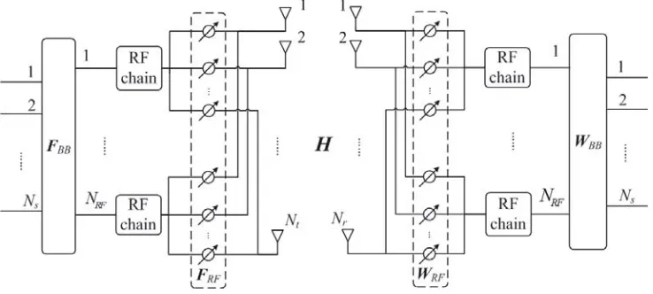
Consider a single-user mm-Wave MIMO system with the hybrid precoder and combiner as shown in Fig. 1, where Nt denotes the number of transmit antennas, Nr the number of receive antennas,

and Ns the number of data streams. The number of RF chains is denoted by NRF such that Ns ≤NRF ≤min(Nt, Nr). Without loss of generality, it is assumed that the transmitter and receiver

have the same number of RF chains. F_RF ∈ CNt×NRF _{represents the analog precoding matrix, and}

FBB ∈CNRF×Ns is the digital precoding matrix. The transmitted signalx can be written as

x=F_RFF_BBs (1)

wheresis theNs×1 vector of transmitted symbols andE[ssH] = _N1_sI. The normalized transmit power

is imposed byF_RFF_BB2_F =Ns. Then the received signal can be written as

y=√ρW_BBH W_RFH HFRFFBBs+WBBH WRFH n (2)

whereρis the average received power,W_RF theNr×NRF analog combining matrix,WBB theNRF×Ns

digital combining matrix at the receiver, nthe noise drawn from the Gaussian distributionCN(0, σ2_n), and H theNr×Nt channel matrix.

The narrowband Saleh-Valenzuela clustering channel model is adopted to characterize the mm-Wave propagation environment [13], i.e.,

H =

NtNr NclNray

Ncl

i=1

Nray

l=1

αilar(φril, θilr)at(φtil, θilt)H (3)

where Ncl is the number of clusters, Nray the number of the propagation paths in each cluster, αil

the gain of thelth ray in the ith cluster distributed as CN(0,1). a_t(φ_ilt, θ_ilt) and a_r(φr_il, θr_il) denote the transmit array response vector and receive array response vector, respectively. (φr_il, θ_ilr) stands for the azimuth and elevation angles of arriver (AOAs), and (φt_il, θ_ilt) denotes the azimuth and elevation angles of departure (AODs). When a uniform planar array (UPA) is considered, the array response vector of thelth ray in the ith cluster can be expressed as [14]

a(φil, θil) =

1 · · · ej2λπd(psinφilsinθil+qcosθil) _{· · · e}j2_λπd((M−1) sinφilsinθil+(N−1) cosθil)T ₍₄₎

where d denotes the antenna spacing; λ represents the signal wavelength; p(0 ≤ p ≤ M) and

q(0≤q≤N) are the antenna indices in the 2-dimensional plane. In matrix form, the channel model in Eq. (3) can be rewritten as

H =

NtNr NclNrayAr

ΛAH_t (5)

whereA_r = [a_r(φr11, θ11r ),· · · ,ar(φrNcl,Nray, θrNcl,Nray)] andAt= [at(φt, θt11),· · ·,at(φtNcl,Nray, θNtcl,Nray)]

are the array response matrices of transmitter and receiver respectively. Λ= diag{α11,· · ·, αNcl,Nray}

is a diagonal matrix.

When the Gaussian symbols are transmitted throughout the mm-Wave channel, the achieved spectral efficiency R can be given by [15]

R= log₂I_Ns+ ρ

NsR

−1

n WBBH WRFH HFRFFBBFBBH FRFH HHWRFWBB

(6)

where R_n = σ_n2W_BBH W_RFH WRFWBB is the noise covariance matrix after the receiving processing.

Furthermore, all the elements of F_RF and W_RF should satisfy the unit modulus constraints, namely,

|FRF(m,n)|=|WRF(m,n)|= 1.

Note that directly maximizing spectral efficiencyRrequires a joint optimization over the four matrix variables (F_RF,FBB,WRF,WBB). However, it is intractable to find the global optimal solution of the

joint optimization problem. Fortunately, the joint design problem can be approximately separated into two sub-problems [12], that is, the precoding and combining problems that have similar mathematical formulations. This paper will mainly focus on the precoding problem, and the presented algorithm can be used to solve the combining problem equivalently.

The precoder optimization problem can be expressed as [16]

arg min

FRF,FBB

Fopt−FRFFBB2F s.t. |FRF(m,n)|= 1, FRFFBB2_F =Ns (7)

where Fopt is the unconstrained fully digital precoder that can be obtained from the SVD of the channel H = UΣVH, i.e., Fopt = VH. |F_RF(m,n)| = 1 is the unit modulus constraint, and

FRFFBB2F = Ns denotes the transmit power constraint. Finding the optimal analytical solutions

of Eq. (7) is still intractable due to the unit modulus constraint of F_RF, and Section 3 will further analyze the optimization problem.

3. ALGORITHM FORMULATION

3.1. Analog Precoding Matrix Refinement

Let’s start with the initialization of the hybrid precoding matrix. As stated above, the hybrid precoding matrix is initialized with the OMP-based sparse hybrid algorithm in [12]. Essentially, the above initialization problem can be considered as a sparse signal reconstruction problem, which is solved with sparse signal recovery methods. According to the compressed sensing theory, the dictionary plays an important role in the OMP method, which can be obtained by either an analytical or a learning-based approach. The analytical approach generates the dictionary via a predefined mathematical transform, while for the learning-based approach, the dictionary is adapted from a set of training signals. Learned dictionaries have potential to improve the performance of the sparse signal recovery algorithms (e.g., the OMP algorithm) further, since the learned dictionaries can capture the salient information directly from the training signals [17]. Therefore, in this section, a novel design is proposed to reduce the residual of the hybrid precoder through refining the matrix F_RF iteratively. The residual β between the optimal precoder Fopt and the hybrid precoder F_RFF_BB can be given by

β =Fopt−F_RFF_BB2_F =

Fopt−

NRF

i=1 fi

RFfBBi

2

F

(8)

wheref_RFi (1≤i≤NRF) is theith column vector of matrix FRF, andf_BBi (1≤i≤NRF) denotes the ith row vector of matrixF_BB. In the refinement stage ofF_RF, the column vectors ofF_RF are modified one by one to reduce the coherence among them [18].

For thei0th column ofF_RF and the correspondingi0th row ofFBB, the optimization problem can

be expressed as

arg min

fi0

RF,fBBi0

Fopt−

NRF

i=i0 fi

RFfBBi −fRFi0 fBBi0

2

F

. (9)

LetG_i0 =Fopt−N_i=RF_i

0 fRFi fBBi , the problem in Eq. (9) can be rewritten as

arg min

fi0

RF,fBBi0

_G

i0 −fRFi0 fBBi0

2

F . (10)

Ignoring the unit modulus constraint temporarily, the optimal solution of the problem in Eq. (10) can be given by the Eckart-Young-Mirsky theorem [19], i.e.,

arg min

fi0

RF,fBBi0

_G

i0−f_RFi0 f_BBi0 2

F =

_Gi0−σ1u1vH

1 2

F (11)

where σ1 is the largest singular value of Gi0, and u1 and v1 are the left and right singular vectors corresponding toσ1. By Eq. (11), f_RFi0 and f_BBi0 can be refined by the following equations

fi0

RF =u1, fBBi0 =σ1v1H. (12)

After the refinement of all the column vectors ofF_RF and the row vectors ofF_BB, the constrained RF precoding matrixF_RF can be given by F_RF(m,n)= _|F_FRF_RF(_(m,nm,n)_)|,∀m, n [20].

3.2. Estimation of the Dominant Singular Value and the Corresponding Singular Vectors

Theorem 1: Suppose thatGis an m×nmatrix with singular valuesσ1> σ2 ≥. . .≥σr>0 and

dominant singular vectors u1 and v1. For the vector sequence

⎧ ⎪ ⎪ ⎨ ⎪ ⎪ ⎩

bk−1 = _GaGak−1

k−12

ak= G H_b

k−1

GHb_k−12

k= 1,2,· · ·, (13)

if aH₀ v1=α1 = 0, then the following statements are true:

(a) lim

k→∞ak= α1

|α1|v1,

(b) lim

k→∞bk = α1

|α1|u1,

(c) lim

k→∞Gak2 =σ1.

Proof: Let the SVD of G ∈ Cm×n be G = UΣVH, where U = [u1 u2 · · · u_m], V =

[v1 v2 · · · vn],Σ=

Σ1 0

0 0

and Σ1= diag{σ1, σ2,· · · , σr}. Decomposinga0 intoa0 =

_n

i=1αivi

(α1=aH0 v1= 0), from Eq. (13), ak and bk can be written as:

ak= G H_b

k−1

GH_b k−12

= G

H_Ga k−1

Gak−12G

H_Gak−1

Gak−122

= G

H_Ga k−1

GH_Ga k−12

= (G

H_G)k_a0

(GH_G)k_a02 =

(VΣ2VH)ka0

(VΣ2_VH₎k_a02

= (

_r

i=1viσi2vHi )ka0

(r_i=1v_iσ_i2v_iH)ka0₂ =

(r_i=1v_iσ2k i vHi )(

_n

i=1αivi)

(r_i=1v_iσ_i2kv_iH)(n_i=1αivi)2 =

_r

i=1αiσi2kvi

r

i=1αiσ2ikvi2

= α1σ 2k

1 (v1+

_r

i=2 ααi1(

σi

σ1) 2k_v

i)

α1σ21k(v1+

_r

i=2_αα₁i(_σσi₁)2kvi)2

bk = _GaGak k2

= GG

H_b k−1

GHb_k−12GGHbk−1

GH_bk−122

= GG

H_b k−1

GGHb_k−12 =

(GGH)kb0

(GGH₎kb0₂ =

(UΣ2UH)kb0

(UΣ2UH₎kb0₂

= (

_r

i=1uiσi2uHi )kGa0

(r_i=1u_iσ2

iuHi )kGa02 = (

_r

i=1uiσi2kuHi )(

_r

i=1αiσiui)

(r_i=1u_iσ2_iku_iH)(r_i=1αiσiui)2 =

_r

i=1αiσi2k+1ui

r

i=1αiσi2k+1ui2

= α1σ 2k+1 1 (u1+

_r

i=2 _αα₁i(_σσ₁i)2k+1ui)

α1σ21k+1(u1+

_r

i=2_αα₁i(_σσ₁i)2k+1ui)2

It is well known that lim

k→∞

σi

σ1

_k

= 0, therefore,

lim

k→∞ak= limk→∞

α1σ12kv1

α1σ21kv12 = α1

|α1|v1,

lim

k→∞bk= limk→∞

α1σ21k+1u1

α1σ12k+1u12 = α1

|α1|u1

(14)

According to Eq. (14), it is clear that

lim

k→∞||Gak||2 =||Gv1||2 =||UΣV H_v1||

2 =

r

i=1

uiσivHi

v1 2

=||σ1u1||2 =σ1.

This concludes the proof.

According to Theorem 1, the extend power algorithm is given in Table 1, where η is the terminal threshold.

3.3. Summary of the P-OMP-IR Algorithm

Table 1. The extended power algorithm.

Input: G, a0, η

Initializations: k= 0

repeat

1: k=k+ 1 2: b_k−1 = _||GaGa_kk₋−₁1_||2

3: a_k = _||GG_HH_bbk−1

k−1||2

untila_k−a_k−12 ≤η 4: σ1 =Gak2

Output: u1 =b_k,v1=a_k,σ1

Table 2. P-OMP-IR algorithm.

Input: Fopt, NRF, At, ε

Initializations: Fres=Fopt, F_RF(0) =A_t, t= 0

repeat

1: F_RF = EmptyMatrix

for j= 1→NRF do

2: Φ=F_RF(t)HFres

3: k= arg max(diag(ΦΦH)) 4: F_RF =

FRF|F_RF(t)(:,k)

5: F_BB(t) = (F_RFH F_RF)−1F_RFH Fopt

6: Fres= Fopt−FRFF (t)

BB

Fopt−FRFF_BB(t)F

end for

7: F_RF(t) =F_RF

8: δt=Fopt−F_RF(t)F_BB(t)_F

Refinement of analog precoder for i= 1→NRF do

9: G_i=Fopt−N_n=RF_i F_RF(t)_(:,n)F_BB(t)_(n,:)

10: Computeu1,v1 and σ1 of Gi by the extended power method

11: F_RF(t)_(:,i) =u1,F_BB(t)_(i,:) =σ1vH1

end for

12: t=t+ 1

13: F_RF(t)_(m,n) = F (t−1)

RF(m,n)

|F_RF(t−₍1)_m,n)|,∀m, n

until (δt−1−δt)≤ε

14: F_BB=√Ns F

(t)

BB

||F_RF(t)F_BB(t)||F

Output: F_RF =F_RF(t), F_BB

4. SIMULATION RESULTS

In this section, several simulation results are presented to evaluate the performance of the proposed hybrid precoding algorithm for a single-user 144×36 mm-Wave MIMO system.

The mm-Wave propagation channel is modeled by L= 50 paths which are equally divided into 5 clustersC_i (i= 1,2,· · · ,5), and each cluster contains 10 rays. The average azimuth and elevation AODs of each cluster, i.e.,φt_Ci = ₁₀1 _l∈C

iφtl,θCti =

1 10

l∈Ciθlt(i= 1,2,· · · ,5), distribute uniformly in (0,2π).

The azimuth and elevation AODs of rays in each cluster are drawn from Laplace distribution, i.e.,

φt_l,l∈Ci ∼ L(μt_φ,Ci, b_φ,t _Ci), θ_l,lt _∈Ci ∼ L(μt_θ,Ci, bt_θ,Ci), where the location parameters μt_φ,Ci =φ_Ct_i, μt_θ,Ci =θt_Ci, and the scale parametersbt_φ,Ci andbt_θ,Ci are set as 10◦. The statistic properties of azimuth and elevation AOAs are the same as the azimuth and elevation AODs. All the results are averaged over 1000 random channel realizations.

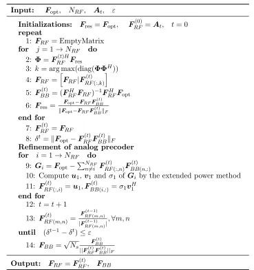
Figure 2 compares the proposed algorithm with the OMP-based sparse precoding algorithm in [12], the successive refinement (SR)-OMP-based sparse precoding algorithm in [22], the PE-AltMin algorithm in [16] and the optimal full digital precoding when SNR = 0 dB, andNs= 4. It is clear that the proposed

algorithm achieves better performance than other hybrid precoders, which implies that the proposed refinement process is effective for reducing the residual of the hybrid precoder. Besides, more RF chains can reduce the performance gap between the proposed algorithm and the full digital precoder remarkably, since more degrees of freedom can be used as the the number of RF chains increases.

4 6 8 10 12 14 16

N_RF 24

25 26 27 28 29 30 31

Spectral Efficiency (bits/s/Hz) Full digital precoding

OMP-based sparse hybrid precoding SR-OMP-based sparse hybrid precoding Proposed P-OMP-IR hybrid precoding PE-AltMin hybrid precoding

Figure 2. Spectral efficiencies given by different algorithms as functions of the number of RF chains NRF when SNR = 0 dB and Ns = 4.

4 4.5 5 5.5 6 6.5 7 7.5 8

N_S 28

30 32 34 36 38 40 42 44 46

Spectral Efficiency (bits/s/Hz) Full digital precoding

OMP-based sparse hybrid precoding SR-OMP-based sparse hybrid precoding Proposed P-OMP-IR hybrid precoding PE-AltMin hybrid precoding

Figure 3. Spectral efficiencies given by different algorithms as functions of the number of data streamsNs when SNR = 0 dB and NRF = 8.

Figure 3 shows spectral efficiency curves with different numbers of data streams Ns, when

SNR = 0 dB andNRF = 8. Obviously, the advantage of the proposed algorithm is more significant when Ns is smaller. For the caseNs=NRF = 8, the spectral efficiencies given by the proposed algorithm and

the SR-OMP-based sparse precoding algorithm are almost the same, and the performance deterioration of the proposed precoding is more severe than the full digital precoder. Therefore, for fixed number of RF chains, transmitting relatively less data streams could reduce the performance loss of the hybrid precoder effectively.

Figure 4 gives the residuals of the proposed approach for different numbers of iterations when SNR = 0 dB, Ns = 4, and the number of RF chains varies from 4 to 8. Explicitly, the residuals

0 1 2 3 4 5 6 7 8 9 10 11 12 13 14 15

Iterations

0.1 0.2 0.3 0.4 0.5 0.6 0.7 0.8

Residual

N

RF=4

N

RF=8

Figure 4. Residuals of the proposed hybrid precoding algorithm as functions of the iterations.

-15 -10 -5

SNR (dB) 10

15 20 25 30 35 40

Spectral Efficiency (bits/s/Hz) _{Full digital precoding}

OMP-based sparse hybrid precoding proposed P-OMP-IR precoding with 1 iteration proposed P-OMP-IR precoding with 5 iterations proposed P-OMP-IR precoding with 10 iterations

0 5

Figure 5. Spectral efficiencies given by different algorithms as functions of the SNR and iterations when Ns= 4 and NRF = 6.

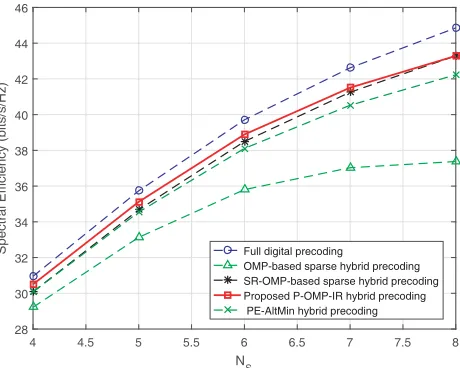
Figure 5 gives the spectral efficiency curves of the proposed method with different iterations when

NRF = 6 and Ns = 4. The optimal full-digital precoding and OMP-based sparse precoding serve as

benchmarks. It can be seen that the spectral efficiency given by the proposed algorithm is improved gradually as the iterations increase. When t = 5, the proposed algorithm can provide about 1 dB SNR gain compared with the OMP-based sparse precoding algorithm. However, if iterations increase continuously, the improvements will be marginal, which means that the proposed algorithm can approach a steady solution with a few iterations.

5. CONCLUSION

In this paper, a hybrid precoding algorithm is proposed for mm-Wave MIMO systems. In the presented approach, the OMP technique is used to initialize the hybrid precoder, then the digital precoding matrix and RF precoding matrix are alternatively refined by the OMP method and the dominant singular vectors given by the extend power method. Simulation results show that the proposed algorithm can not only approach a steady solution with a few iterations, but also offer higher spectral efficiencies than existing sparse precoding algorithms.

ACKNOWLEDGMENT

This work was supported by the Natural Science Foundation of Hebei Province (No. F2016501139), the Fundamental Research Funds for the Central Universities under Grant (Grant No. N172302002, Grant No. N162304002), and the National Natural Science Foundation of China (Grant No. 61501102, Grant No. 61473066).

REFERENCES

1. Kutty, S. and D. Sen, “Beamforming for millimeter wave communications: An inclusive survey,”

IEEE Commun. Surveys Tuts., Vol. 18, No. 2, 949–973, 2016.

2. Heath, R. W., N. Gonzalez-Prelcic, Jr., S. Rangan, W. Roh, and A. M. Sayeed, “An overview of signal processing techniques for millimeter wave MIMO systems,” IEEE J. Sel. Topics Signal

3. Han, S., I. Chih-Lin, Z. Xu, and C. Rowell, “Large-scale antenna systems with hybrid analog and digital beamforming for millimeter wave 5G,”IEEE Commun. Mag., Vol. 53, No. 1, 186–194, 2015. 4. Kanatas, A. G., “A receive antenna subarray formation algorithm for MIMO systems,” IEEE

Commun. Lett., Vol. 11, No. 5, 1396–1398, 2007.

5. Venkateswaran, V. and A. J. Veen, “Analog beamforming in MIMO communications with phase shift networks and online channel estimation,” IEEE Trans. Signal Process., Vol. 58, No. 8, 4131– 4143, 2010.

6. Nsenga, J., A. Bourdoux, W. V. Thillo, V. Ramon, and F. Horlin, “Joint Tx/Rx analog linear transformation for maximizing the capacity at 60 GHz,” IEEE Int. Conf. Commun., 1–5, 2011. 7. Ni, W., X. Dong, and W. S. Lu, “Near-optimal hybrid processing for massive MIMO systems via

matrix decomposition,” IEEE Trans. Signal Process., Vol. 65, No. 15, 3922–3933, 2017.

8. Singh, J. and S. Ramakrishna, “On the feasibility of codebook-based beamforming in millimeter wave systems with multiple antenna arrays,” IEEE Trans. Wireless Commun., Vol. 14, No. 5, 2670–2683, 2015.

9. Dai, L., X. Gao, J. Quan, S. Han, and I. Chih-Lin, “Near-optimal hybrid analog and digital precoding for downlink mmWave massive MIMO systems,”Proc. IEEE Int. Conf. Commun., 1334– 1339, 2015.

10. Raghavan, V., S. Subramanian, J. Cezanne, and A. Sampath, “Directional beamforming for millimeter-wave MIMO systems,” IEEE Global Commun. Conf., 1–7, 2015.

11. Alkhateeb, A., O. E. Ayach, G. Leus, and R. W. Heath, “Hybrid precoding for millimeter wave cellular systems with partial channel knowledge,”Inf. Theory Appl. Workshop, 1–5, 2013.

12. Ayach, O. E., S. Rajagopal, S. Abu-Surra, Z. Pi, and R. W. Heath, “Spatially sparse precoding in millimeter wave MIMO systems,” IEEE Trans. Wireless Commun., Vol. 13, No. 3, 1499–1513, 2014.

13. Rusu, C., R. Mendez-Rial, N. Gonzalez-Prelcic, and R. W. Heath, “Low complexity hybrid precoding strategies for millimeter wave communication systems,”IEEE Trans. Wireless Commun., Vol. 15, No. 12, 8380–8393, 2016.

14. Balanis, C., Antenna Theory, Wiley, 1997.

15. Alkhateeb, A., O. E. Ayach, G. Leus, and R. W. Heath, “Hybrid precoding for millimeter wave cellular systems with partial channel knowledge,”IEEE Inf. Theory Appl. Workshop, 1–5, 2013. 16. Yu, X., J. C. Shen, J. Zhang, and K. B. Letaief, “Alternating minimization algorithms for hybrid

precoding in millimeter wave MIMO systems,”IEEE J. Sel. Topics Signal Process., Vol. 10, No. 3, 485–500, 2016.

17. Wei, D., T. Xu, and W. Wang, “Simultaneous codeword optimization (SimCO) for dictionary update and learning,”IEEE Trans. Signal Process., Vol. 60, No. 12, 6340–6353, 2011.

18. Aharon, M., M. Elad, and A. Bruckstein, “K-SVD: An algorithm for designing overcomplete dictionaries for sparse representation,” IEEE Trans. Signal Process., Vol. 54, No. 11, 4311–4322, 2006.

19. Wei, M., “Perturbation theory for the Eckart-Young-Mirsky theorem and the constrained total least squares problem,” Linear Algebra Appl., Vol. 280, No. 2, 267–287, 1998.

20. Alkhateeb, A. and R. W. Heath, “Frequency selective hybrid precoding for limited feedback millimeter wave systems,” IEEE Trans. Commun., Vol. 64, No. 5, 1801–1818, 2016.

21. Liu, F. L., R. Y. Du, J. P. Guo, and S. M. Guo, “P-GLRT algorithm for cooperative spectrum sensing,”Wireless Personal Commun., Vol. 81, No. 3, 1079–1089, 2015.