Article
1
Grey relational analysis for hesitant fuzzy sets and
2
interval-valued hesitant fuzzy sets with applications
3
to MADM problems
4
Xin Guan, Guidong Sun*, Xiao Yi*, Jing Zhao
5
Department of Electronics and Information Engineering, Naval Aeronautical and Astronautical University,
6
Yantai 264001, China; [email protected]
7
* Correspondence: [email protected], [email protected]; Tel.: +86-13001603600
8
Abstract: Quantitative and qualitative fuzzy measures have been proposed to hesitant fuzzy sets
9
(HFSs) from different points. However, few of the existing HFSs fuzzy measures refer to the grey
10
relational analysis (GRA) theory. Actually, the GRA theory is very useful in the fuzzy measure
11
domain, which has been developed for such the intuitionistic fuzzy sets. Therefore, in this paper,
12
we apply the GRA theory to the HFSs and interval-valued hesitant fuzzy sets (IVHFS) domain. We
13
propose the HFSs grey relational degree, HFSs slope grey relational degree, HFSs synthetic grey
14
relational degree and IVHFSs grey relational degree, which describe the closeness, the variation
15
tendency and both the closeness and variation tendency of HFSs and closeness of IVHFSs,
16
respectively, greatly enriching the fuzzy measures of HFSs. Furthermore, with the help of the
17
TOPSIS method, we develop the grey relational based MADM methodology to solve the HFSs and
18
IVHFSs MADM problems. Finally, combined with two practical MADM examples about energy
19
policy selection with HFSs information and emergency management evaluation with IVHFSs
20
information, we obtain the most desirable decision results, and compared with the previous
21
methods, the validity, effectiveness and accuracy of the proposed grey relational degree for HFSs
22
and IVHFSs are demonstrated in detail.
23
Keywords: Grey relational analysis (GRA); Hesitant Fuzzy Sets (HFSs); Interval-valued hesitant
24
fuzzy sets (IVHFS); grey relational degree; grey relational based MADM methodology
25
26
1. Introduction
27
The introduction should briefly place the study in a broad context and highlight why it is
28
important. It should define the purpose of the work and its significance. The current state of the
29
research field should be reviewed carefully and key publications cited. Please highlight
30
controversial and diverging hypotheses when necessary. Finally, briefly mention the main aim of the
31
work and highlight the principal conclusions. As far as possible, please keep the introduction
32
comprehensible to scientists outside your particular field of research. References should be
33
numbered in order of appearance and indicated by a numeral or numerals in square brackets, e.g.,
34
[1] or [2,3], or [4–6]. See the end of the document for further details on references.
35
In 2009, Torra [1, 2] originally introduced the hesitant fuzzy sets (HFSs) and several basic
36
operations for it. HFSs is one of the most efficient decision making techniques to deal with imprecise
37
and vague information and a growing number of studies focus on not only the properties but also
38
the applications of it.
39
Xia and Xu [3, 4], Liao and Xu [5, 6] first introduced some basic operations, aggregation
40
operators, score function and variance for HFSs. Afterwards, Xu and Xia [7-9] proposed a variety of
41
distance, similarity, entropy and correlation measures for hesitant fuzzy sets. Farhadinia [10] also
42
investigated the relationship between the distance, similarity and entropy measure for HFSs and
43
developed division and subtraction formulas for HFSs [11]. Li, Zeng and Zhao [12] introduced the
44
concept of hesitance degree for HFE and presented some new distance measures between HFSs
45
which contained the hesitance degrees, later they applied these new distances to solve pattern
46
recognition problems [13]. Zhao, Xu and Liu [14] proposed a new axiomatic framework of entropy
47
measures for HFEs by taking fully into account two faces of uncertainty associated with an HFE.
48
Chen, Xu and Xia [15], Liao, Xu and Zeng [16] proposed some novel correlation coefficients of
49
hesitant fuzzy sets for clustering analysis and medical diagnosis.
50
Besides a variety of operations, properties and fuzzy measures on HFSs, the hesitant fuzzy sets
51
has shown its advantages in such the real fields as decision-making [3, 4, 6, 9 16-21], feature selection
52
[22], pattern recognition [13], cluster analysis [15, 16] and linguistic computing [23-25]. He et al [17]
53
first introduced the expected value and the geometric average value of hesitant multiplicative
54
element (HME) to group decision making problems. Xu and Zhang [18] developed a novel approach
55
based on TOPSIS and the maximizing deviation method for solving MADM problems with hesitant
56
fuzzy information. Qin, Liu and Pedrycz [19] investigated multiple attribute decision making
57
(MADM) problems with hesitant fuzzy attribute based on Frank triangular norms. Zhang et al [20]
58
proposed an interval programming method for solving MAGDM problems with hesitant fuzzy
59
alternatives based on LINMAP. Ashtiani and Azgomi [21] proposed a hesitant fuzzy multi-criteria
60
decision making based computational trust model capable of taking into account the fundamental
61
building blocks corresponding to the concept of trust. Ebrahimpour and Eftekhari [22] proposed an
62
innovative method to deal with feature subset selection with HFSs based on Maximum Relevancy
63
and Minimum Redundancy approach. Rodríguez, Martínez and Herrera et al [23] introduced the
64
concept of a hesitant fuzzy linguistic term set (HLFSs) to provide a linguistic and computational
65
basis. Liao et al [24] developed a method to solve the MCDM problem within the context of HLFSs.
66
Wang et al [25] developed a likelihood-based TODIM approach for the selection and evaluation with
67
multi-hesitant fuzzy linguistic information.
68
Chen, Xu and Xia [26] extended the HFSs and first introduced the interval-valued hesitant
69
fuzzy set (IVHFS) to describe uncertain evaluation information in group decision making (GDM)
70
processes, presented some operational laws and a score function for IVHFS and also proposed
71
correlation coefficients for it [15]. Subsequently they [27] derived the properties and relationships of
72
fundamental operations on IVHFSs for Algebraic t-norm and t-conorm and presented the operations
73
based on Archimedean t-norm and t-conorm and investigated their properties. Farhadinia [28, 11]
74
introduced the division and subtraction formulas for IVHFSs and discussed the distance, similarity
75
and entropy measure of IVHFSs and applied into clustering analysis. Fernández, Alonso and
76
Bustince et al [29, 30] introduced finite interval-valued hesitant fuzzy sets, defined a new order,
77
entropy between them considering the fuzziness, lack of knowledge and hesitance and applied in
78
the business selection. Verma [31] proposed four new operations on IVHFS and study their
79
properties and relations in details. Gitinavard, Mousavi and Vahdani [32] introduced a novel
80
multi-criteria weighting and ranking model with interval-valued hesitant fuzzy setting and applied
81
to location and supplier selection problems. Zhang [33] developed two interval-valued hesitant
82
fuzzy QUALIFLEX outranking methods to handle MCDM problems concerning the selection of
83
green suppliers. Jin, Ni and Chen et al [34] developed two interval-valued hesitant fuzzy prioritized
84
aggregation operators with the help of Einstein operations to investigate interval-valued hesitant
85
fuzzy multi-attribute group decision-making problems. Zhang, Li and Mu et al [35] proposed a new
86
rough set model that combines interval-valued hesitant fuzzy sets with multigranulation rough sets
87
over two universes and applied to steam turbine fault diagnosis.
88
Despite of the qualitative and quantitative studies of HFSs and IVHFSs, the present work for
89
them mainly focuses on such fuzzy measures as distance, similarity, entropy and correlation
90
coefficients measure, few studies referred to the critical fuzzy measure over HFSs and IVHFSs: grey
91
relational analysis. Meanwhile the correlation coefficients measure can only calculate the linear
92
fashion of two HFSs and IVHFSs, they can not measure the closeness. Therefore, the applications of
93
the HFSs and IVHFSs correlation coefficients are controversial, they are only one aspect of the real
94
fuzzy measures. For the above reasons, it is essential to apply the grey relational analysis for HFSs
95
Actually, the traditional grey relational analysis of the fuzzy set takes an important occupation
97
in the fuzzy measure field. It can measure the closeness of two fuzzy sets just like the distance and
98
similarity measure. Many researchers have focused on the grey relational analysis of fuzzy set and
99
proposed several approaches to solve decision making problems. Wei [36-39] established a series of
100
grey relational analysis (GRA) method to investigate the multiple attribute decision-making
101
problems with intuitionistic fuzzy information, 2-tuple linguistic information and the dynamic
102
hybrid multiple attribute decision information. Zhang, Liu and Zhai [40], Zhang, Jin and Liu [41],
103
Guo [42] also developed the grey relational analysis method for solving MCDM problems with
104
interval-valued triangular fuzzy numbers, intuitionistic trapezoidal fuzzy number and hybrid
105
multiple attribute information respectively. Kong, Wang and Wu [43] presented a new algorithm
106
based on grey relational analysis to discuss fuzzy soft set decision problems. Kuo and Liang [44]
107
combined the concepts of VIKOR and grey relational analysis to present an effective fuzzy MCDM
108
method. Tang [45], Li, Wen and Xie [46] proposed a novel fuzzy soft set approach in decision
109
making based on grey relational analysis and Dempster-Shafer theory of evidence respectively.
110
Unfortunately, only a few of these grey relational analyses referred to HFSs and IVHFSs, so grey
111
relational analysis for HFSs and IVHFSs is necessary and urgent.Wei and Li [47] establish an
112
optimization model based on GRA to get the weight vector of the HFSs criteria, Sun, Guan, Yi and
113
Zhou [48] defined the difference and slope of the HFSs to form a grey relational degree, which is
114
inspiring to be used in our this paper.
115
Consequently, the motivation of this paper is to extend the concept of grey relational analysis to
116
HFSs and IVHFSs and develop a methodology to solve MADM problems with HFSs and IVHFSs
117
information. The novelties of this paper concentrate on the five aspects: (1) Investigate the grey
118
relational analysis to HFSs and propose the grey relational coefficient and grey relational degree of
119
the HFSs for the first time. (2) Propose the slope grey relational coefficient and slope grey relational
120
degree of the HFSs. (3) Propose the synthetic grey relational coefficient and synthetic grey relational
121
degree of the HFSs. (4) Extend the grey relational analysis to IVHFSs and proposed the grey
122
relational coefficient and grey relational degree of the IVHFSs. (5) Develop a MADM methodology
123
with HFSs and IVHFSs information.
124
The rest of the paper is as follows: Section 2 briefly reviews the concepts of HFSs, IVHFSs and
125
grey relational analysis theory. In Section 3, we define the grey relational coefficient and grey
126
relational degree for HFSs for the first time and propose some extended HFSs grey relational
127
expression as the slope and synthetic grey relational degree. Furthermore, we extend the grey
128
relational analysis to IVHFSs. In Section 4, we develop a hesitant fuzzy MADM methodology based
129
on the grey relational analysis between HFSs and IVHFSs. In Section 5, we apply the proposed grey
130
relational hesitant fuzzy MADM methodology to the practical MADM problems. Finally, the paper
131
ends with some concluding remarks and future challenges in Section 6.
132
2. Preliminaries
133
In this section, we recall the HFSs, IVHFSs and grey relational analysis theory.
134
2.1. Hesitant fuzzy sets and interval-valued hesitant fuzzy sets
135
When an expert makes a decision, he may hesitate to choose the exact membership degree in [0,
136
1]. For such a circumstance where there are several membership degrees of one element to a set,
137
Torra [1, 2] developed the hesitant fuzzy set (HFS), which is a kind of generalized fuzzy set where
138
the membership degree of an element to a certain set can be illustrated as several different values
139
between 0 and 1. HFSs is good at dealing with the situations that people have disagreements or
140
hesitancy when deciding something.
141
Definition 1. [1, 2]. Suppose that X={ , , , }x x1 2 xn is a reference set, a hesitant fuzzy set (HFS)
142
A on X is defined in terms of a function h xA( ) when applied to X returns a subset of [0, 1], i.e.
143
{ , ( )A }
A= x h x x X∈
(1)
Where h xA( ) is a set of some different values in [0, 1], representing the possible membership
145
degrees of the element x X∈ to the set A. For convenience, Xia and Xu [5] call h xA( ) a hesitant
146
fuzzy element (HFE), which is a basic unit of HFS.
147
In many real problems, due to insufficiency in available information, it may be difficult to
148
exactly quantify the attribute with a crisp number, but can be represented by an interval number
149
within [0, 1]. Thus, Chen, Xu and Xia [26] introduced the concept of interval-valued hesitant fuzzy
150
sets (IVHFSs), which permit the membership degrees of an element to a given set to have a few
151
different interval values.
152
Definition 2. [26]. Suppose that X ={ , , , }x x1 2 xn is a reference set, D[0,1] is the set of all closed
153
subintervals of [0, 1]. An interval-valued hesitant fuzzy sets (IVHFSs) A on X is defined as
154
{ , ( )A }
A= x h x x X∈
(2)
155
Where h xA( ) denotes all possible interval-valued membership degrees of the element, is a set of
156
some different values in [0, 1], represents the possible membership degrees of the element x X∈ to
157
the set A. For convenience, they call h xA( ) an interval-valued hesitant fuzzy element (IVHFE),
158
which is a basic unit of IVHFS.
159
( ) { | ( )}
A A
h x = γ γ ∈h x
(3)
160
Where γ is an interval number, γ=[ ,γ γ L U]
, γLand γUrepresent the lower and upper limits of γ,
161
respectively.
162
2.2. Grey relational analysis Theory
163
Grey relational theory was originally introduced by Deng [49]. It has been widely applied to
164
decision making, pattern recognition and some other problems under uncertainty, particularly
165
under the discrete data and fuzzy information.
166
Definition 3. [47]. For reference setX0=(x0(j),j=1,2,,k) and Xi=(xi(j),j=1,2,,k), the grey
167
relational coefficient is defined by
168
0 0
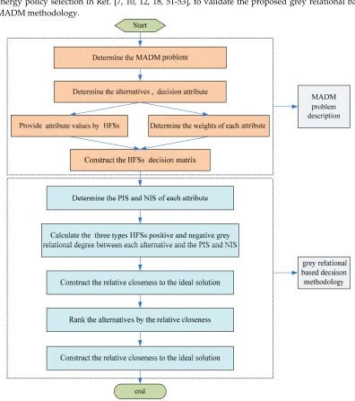
0
0 0
min min ( ) ( ) max max ( ) ( )
( ( ), ( ))
( ) ( ) max max ( ) ( )
i i
i j i j
i
i i j i
x j x j x j x j
r x j x j
x j x j x j x j
ρ ρ
− + ⋅ −
=
− + ⋅ −
(4)
169
Where ρ is the distinguished coefficient, ρ ∈[0,1].
170
The grey relational degree is defined as:
171
0 0
1 1
( , i) k ( ( ), ( ))i
j
X X r x j x j
k
γ
=
= ⋅
(5)
172
Take the weight into consideration, let the weight vector of Xi is w={ ,w w1 2, , wk}, 1
1 k
j j
w =
=
,173
1, 2, ,
j= k, the grey relational degree is extended to the weighted grey relational degree:
174
0 0
1
( , i) k j ( ( ), ( ))i
j
X X w r x j x j
γ
=
=
⋅(6)
175
The traditional grey relational theory describes the closeness of two variables, which is
176
necessary in the decision making and pattern recognition fields. In this paper, we will extend it to
177
the HFSs and IVHFSs domain.
178
3. Grey relational analysis for HFSs and IVHFSs
179
In this section, we apply grey relational theory to the HFSs and IVHFSs domain and define
180
some novel HFSs expressions based on grey relational theory.
181
Definition 4. For two hesitant fuzzy sets on the fixed set X={ , , , }x x1 2 xn ,
183
{
i, ( ) |A i i , 1, 2, ,}
A= x h x x ∈X i= n and Bj =
{
x hi, Bj( ) |xi xi∈X i, =1, 2, , , n j=1, 2, , m}
with184
{
1 2}
( )= , , , Ai
A i Ai Ai Ail
h x γ γ γ , hBj( )=xi
{
γB ij1,γB ij2, ,γB ilj B ij}
, i=1, 2, , n, j=1, 2, , m, then we define185
the grey relational coefficient between HFEs h xA( )i and hBj( )xi as:
186
min min{ ( ( ), ( ))} max max{ ( ( ), ( ))}
( ( ), ( ))
( ( ), ( )) max max{ ( ( ), ( ))}
j j
j
j j
A i B i A i B i
j i j i
A i B i
A i B i j i A i B i
d h x h x d h x h x
r h x h x
d h x h x d h x h x
ρ ρ
+ ⋅ =
+ ⋅
(7)
187
Where d h x h( ( ),A i Bj( ))xi is the distance between HFEs h xA( )i and hBj( )xi , which can be calculated
188
according to following equations:
189
1/2 2
1
1
( ( ), ( )) ( Ai )
j j
l
hne A i B i Aik B ik
k Ai
d h x h x
l = γ γ
= −
(8)
190
Actually, there have been proposed a variety of distance measures for HFEs, for more detail, please
191
refer to reference [7, 8, 11-13].
192
Based on grey relational coefficient between HFEs, the grey relational degree between HFSs A
193
and Bj is defined as:
194
1 1
( , j) n ( ( ),A i Bj( ))i
i
A B r h x h x
n
γ
=
= ⋅
(9)
195
In practical applications, the elements { , , , }x x1 2 xn in the universe X have different weights.
196
Take the weight into consideration, let the weight vector of X is w={ ,w w1 2, ,wn}, 1
1 n
i i
w =
=
,197
1, 2, ,
i= n, we extend the HFSs grey relational degree to the weighted HFSs grey relational degree
198
as:
199
1
( , ) ( ( ), ( ))
j
n
w j i A i B i
i
A B w r h x h x
γ
=
=
⋅ (10)200
3.2. Slope grey relational definition for HFEs and HFSs
201
The HFSs grey relational degree in section 3.1 mainly focus on the closeness of the two HFSs,
202
here we extend a novel HFSs grey relational degree called HFSs slope grey relational degree to
203
represent the linear fashion of HFSs. As a departure, we introduce two new concepts of HFEs and
204
HFSs. Sun et al. [48] defined the difference and slope of the HFSs.
205
Definition 5. [48] For hesitant fuzzy sets A=
{
x h xi, ( ) |A i xi∈X i, =1, 2, , n}
with206
{
1 2}
( )= , , , Ai
A i Ai Ai Ail
h x γ γ γ on the fixed set X={ , , , }x x1 2 xn , we define the difference of the HFSs as
207
{
i, A( ) |i i , 1, 2, ,}
A x h x x X i n
Δ = Δ ∈ =
(11)
208
Where Δh xA( )i denotes the difference of the HFEs.
209
{
1 2 1}
( )= , , , , ,
Ai
A i Ai Ai Aik Ail
h x γ γ γ γ −
Δ Δ Δ Δ Δ
(12)
210
Where
211
1 , 1, 2, , 1
Aik Aik Aik k lAi
γ γ + γ
Δ = − = −
(13)
212
Definition 6. [48] For hesitant fuzzy sets A=
{
x h xi, ( ) |A i xi∈X i, =1, 2, , n}
with213
{
1 2}
( )= , , , Ai
A i Ai Ai Ail
h x γ γ γ on the fixed set X ={ , , , }x x1 2 xn , the difference of A is
214
{
i, A( ) |i i , 1, 2, ,}
A x h x x X i n
Δ = Δ ∈ = with Δh xA( )=i
{
ΔγAi1,ΔγAi2, , ΔγAik, , ΔγAilAi−1}
, we define the215
slope of the HFSs as
216
{
'}
' , ( ) | , 1, 2, ,
i A i i
A = x h x x ∈X i= n
(14)
217
{
}
'( )= '1, '2, , ' , , ' 1
Ai
i
A A i A i A ik A il
h x γ γ γ γ −
(15)
219
Where
220
' 1 , 1, 2, , 1
( ) ( )
Aik Aik Aik
Ai A ik
A i A i
k l
h x h x
γ γ γ
γ = Δ = + − = −
(16)
221
Where h xA( )i is the mean of the HFE h xA( )i
222
1 1
( ) Ai
l
A i Aik
k Ai h x
l = γ
=
,
i=1, 2, , n(17)
223
The difference and slope of the HFSs can denote the linear fashion of the HFSs clearly, which is
224
useful in practice. Based on the two concepts, we give the a novelHFSs slope grey relational
225
coefficient, which extends Sun et al.’s definition [48].
226
Definition 7. For two hesitant fuzzy sets on the fixed set X={ , , , }x x1 2 xn ,
227
{
i, ( ) |A i i , 1, 2, ,}
A= x h x x ∈X i= n and Bj =
{
x hi, Bj( ) |xi xi∈X i, =1, 2, , , n j=1, 2, , m}
with228
{
1 2}
( )= , , , Ai
A i Ai Ai Ail
h x γ γ γ , hBj( )=xi
{
γB ij1,γB ij2, , γB ilj B ij}
, i=1, 2, , n, j=1, 2, , m, the difference of229
them are Δ =A
{
xi,Δh xA( ) |i xi∈X i, =1, 2, , n}
, Δh xA( )=i{
ΔγAi1,ΔγAi2, , ΔγAik, , ΔγAilAi−1}
,230
1 Aik Aik Aik
γ γ + γ
Δ = − , k=1, 2, , lAi−1 and Δ =Bj
{
xi,ΔhBj( ) |xi xi∈X i, =1, 2, , , n j=1, 2, , m}
,231
{
1 2 1}
( )= , , , , ,
j j j j j B ij
B i B i B i B ik B il
h x γ γ γ γ −
Δ Δ Δ Δ Δ , ΔγB ikj =γB ikj +1−γB ikj , k=1, 2, ,lB ij −1, the slope of
232
them are
{
'}
' , ( ) | , 1, 2, ,
i A i i
A = x h x x ∈X i= n with '( )=
{
'1, '2, , ' , , ' 1}
Ai
i
A A i A i A ik A il
h x γ γ γ γ − and
233
{
'}
'
, ( ) | , 1, 2, ,
j
j i B i i
B = x h x x ∈X i= n with '( )=
{
'1, '2, , ' , , ' 1}
j i j j j j Ai
B B i B i B ik B il
h x γ γ γ γ − , we define the HFSs
234
slope grey relational coefficient between the HFEs h xA( )i and hBj( )xi as:
235
1 1 1 ( ( ), ( )) ( ( ), ( )) 1 Ai j j ls A i B i s A i B i
k Ai
r h x h x h x h x
l ξ
−
=
= Δ Δ
−
(18)
236
Where237
' ' ' ' ' ' ' 1 1 1 1 11 ( )
( ( ), ( )) 1 1 ( ) ( ) ( ) j j j j j Aik Aik
A ik A i
s A i B i
B ik B ik A ik A ik B ik Aik Aik Aik Aik
A i A i B i
h x
h x h x
h x h x h x
γ γ γ ξ γ γ γ γ γ γ γ γ γ + + + + − + + Δ Δ = = − + + − + − + − −
(19)
238
Based on HFSs slope grey relational coefficient, the HFSs slope grey relational degree is defined as:
239
1 1
( , ) n ( ( ), j( ))
s j s A i B i
i
A B r h x h x
n
γ
=
= ⋅
(20)
240
Take the weight into consideration, let the weight vector of X is w={ ,w w1 2, ,wn}, 1 1 n i i w = =
,241
1, 2, ,
i= n, we extend the HFSs slope grey relational degree to the weighted HFSs slope grey
242
relational degree as:
243
1
( , ) n ( ( ), j( ))
sw j i s A i B i
i
A B w r h x h x
γ
=
=
⋅ (21)244
3.3. Synthetic grey relational definition for HFSs
245
Definition 8. For two hesitant fuzzy sets on the fixed set X={ , , , }x x1 2 xn ,
246
{
i, ( ) |A i i , 1, 2, ,}
A= x h x x ∈X i= n and Bj =
{
x hi, Bj( ) |xi xi∈X i, =1, 2, , , n j=1, 2, , m}
with247
{
1 2}
( )= , , , Ai
A i Ai Ai Ail
h x γ γ γ , hBj( )=xi
{
γB ij1,γB ij2, ,γB ilj B ij}
, the slope of them are248
{
'}
' , ( ) | , 1, 2, ,
i A i i
A = x h x x ∈X i= n with '( )=
{
'1, '2, , ' , , ' 1}
Ai
i
A A i A i A ik A il
h x γ γ γ γ − and
{
'}
' , ( ) | , 1, 2, ,
j
j i B i i
B = x h x x ∈X i= n with '( )=
{
'1, '2, , ' , , ' 1}
j i j j j j Ai
B B i B i B ik B il
h x γ γ γ γ − , i=1, 2, , n ,
250
1, 2, ,
j= m, then we define the HFEs synthetic grey relational coefficient between HFEs h xA( )i
251
and hBj( )xi as:
252
' '
' ' ' '
1 2
( ( ), ( ))
1 max max{ ( ( ), ( ))} max max{ ( ( ), ( ))}
1 ( ( ), ( )) ( ( ), ( )) max max{ ( ( ), ( ))} max max{ ( ( ), ( ))}
j
j j
j j j j
c A i B i
A i B i A i B i
i j i
j
A i B i A i B i j i A i B i j i A i B i
r h x h x
d h x h x d h x h x
d h x h x d h x h x d h x h x d h x h x
ξ η
λ λ ξ η
=
+ ⋅ + ⋅
+ ⋅ + ⋅ + ⋅ + ⋅
253
(22)
254
Where λ λ >1, 1 0, which indicate the importance of the closeness and linear fashion of HFSs,
255
respectively, which satisfied λ λ1+ 2=1, ξ and η denote the distinguished coefficient of the
256
closeness and linear fashion, d h x h( ( ),A i Bj( ))xi and ( '( ), '( ))
j
i i
A B
d h x h x are the distance between HFEs
257
( ) A i
h x and hBj( )xi and the distance between the slope of HFEs h xA( )i and hBj( )xi , respectively,
258
' '
( ( ), ( ))
j
i i
A B
d h x h x can be calculated by
259
' ' ' '
1/2
1 2
1
1
( ( ), ( )) ( )
1
Ai
j j
l
hne A i B i A ik B ik
k Ai
d h x h x
l γ γ
−
=
= −
−
(23)260
If the numbers of values in different HFEs of HFSs are different, we have to extend the shorter one
261
until both of them have the same length when we compare them. We can extend them according to
262
the optimistic or the pessimistic methods in [7,8].
263
Based on HFEs synthetic grey relational coefficient, the HFSs synthetic grey relational degree is
264
defined as:
265
1 1
( , ) n ( ( ), j( ))
c j c A i B i
i
A B r h x h x
n
γ
=
= ⋅
(24)
266
Take the weight into consideration, let the weight vector of X is w={ ,w w1 2, ,wn}, 1
1 n
i i
w =
=
,267
1, 2, ,
i= n, we extend the HFSs synthetic grey relational degree to the weighted HFEs synthetic
268
grey relational degree as:
269
1
( , ) n ( ( ), j( ))
cw j i c A i B i
i
A B w r h x h x
γ
=
=
⋅(25)
270
The HFSs synthetic grey relational degree takes the considerations of both the closeness and
271
linear fashion of HFSs together, which can better represent the fuzzy measure between the HFSs.
272
3.4. Grey relational definition of IVHFEs and IVHFSs
273
An interval-valued hesitant fuzzy sets (IVHFSs) A on X is defined as
274
{ , ( )A }
A= x h x x X∈
(26)
275
Where h xA( ) denotes all possible interval-valued membership degrees of the element is a set of
276
some different values in [0, 1], representing the possible membership degrees of the element x X∈
277
to the set A. For convenience, they call h xA( ) an interval-valued hesitant fuzzy element (IVHFE),
278
which is a basic unit of IVHFS.
279
( ) { | ( )}
A A
h x = γ γ ∈h x
(27)
280
Here γ is an interval number, γ=[ ,γ γ L U], γLand γUrepresent the lower and upper limits of γ,
281
Definition 9. For two interval-valued hesitant fuzzy sets on the fixed set X={ , , , }x x1 2 xn ,
283
{ , ( )A i i , 1, 2, , }
A= x h x x ∈X i= n and
{
, ( ) | , 1, 2, , , 1, 2, ,}
j
j i B i i
B = x h x x ∈X i= n j= m with
284
{
1 2}
( )= , , ,
Ai
i
A Ai Ai Ail
h x γ γ γ
,
{
}
1 2
( )= , , ,
j j j j B ij
B i B i B i B il
h x γ γ γ
, i=1, 2, , n, j=1, 2, , m, then we define
285
the grey relational coefficient between HFEs h xA( )i and hBj( )xi as:
286
min min{ ( ( ), ( ))} max max{ ( ( ), ( ))}
( ( ), ( ))
( ( ), ( )) max max{ ( ( ), ( ))}
j j
j
j j
i B i i B i
A A
j i j i
i B i A
i B i i B i
A j i A
d h x h x d h x h x
r h x h x
d h x h x d h x h x
ρ ρ + ⋅ = + ⋅
(28)
287
Where d h x h( ( ),A i Bj( ))xi is the distance between IVHFEs h xA( )i and hBj( )xi , which can be
288
calculated according by
289
1/2 2 2 1 1 ( ( ), ( )) ( ) 2 Aij j j
l
L L U U
hne A i B i Aik B ik Aik B ik
k Ai
d h x h x
l = γ γ γ γ
= − + −
(29)
290
For more distance between IVHFEs, please refer to Ref. [11, 26-31].
291
Based on grey relational coefficient between IVHFEs, the grey relational degree between
292
IVHFSs A and Bj is defined as:
293
1 1
( , j) n ( ( ),A i Bj( ))i
i
A B r h x h x
n
γ
=
= ⋅
(30)
294
Take the weight into consideration, let the weight vector of X is w={ ,w w1 2, ,wn}, 1 1 n i i w = =
,295
1, 2, ,
i= n, we extend the IVHFSs grey relational degree to the weighted IVHFSs grey relational
296
degree as:
297
1
( , ) n ( ( ), j( ))
w j i A i B i
i
A B w r h x h x
γ
=
=
⋅
(31)
298
4. The grey relational based MADM methodology with HFSs and IVHFSs information
299
In this section, we investigate the grey relational analysis to MADM problems with HFSs and
300
IVHFSs information, and propose the grey relational based MADM methodology with the help of
301
the TOPSIS [50] method.
302
Suppose that a hesitant fuzzy MADM problem has m alternativesA ii( =1, 2, , ) m , each
303
alternative have n hesitant fuzzy attribute C jj( =1, 2, , ) n , denote
304
{
1 2}
( )= , , , , ,
i i i i i ij
A j A A A k A l
h C γ γ γ γ represent the hesitant fuzzy information of the alternatives Ai on
305
the attribute Cj, lij is the number of the membership values in h CAi( )j , let w={ ,w w1 2, , wn}be
306
the relative weight vector of the attribute, satisfying the normalization conditions: 0≤wj≤1 and
307
1 1 n j j w = =
. Then all the hesitant fuzzy information can be concisely expressed in matrix format as:308
1 1 1
2 2 1 2 1 1 2 ( ) ( ) ( ) ( ) ( ) ( ) ( ) ( ) ( ) i
m m m
A A A n
A A n
A j
A A A n m n
h C h C h C
h C h C
h C
h C h C h C
× =
A
(32)
309
Then according to the TOPSIS approach, we propose the grey relational based MADM methodology
310
with hesitant fuzzy matrix as follows:
311
Step 1: Determine the positive ideal solution (PIS) and negative ideal solution (NIS) of each attribute
312
{
j, A( ) |j j , 1, 2, ,}
A+ = C h C+ C ∈C j= n
(33)
314
{
j, A( ) |j j , 1, 2, ,}
A− = C h C− C ∈C j= n
(34)
315
Where h CA+( )j and h CA−( )j are the new positive and negative HFEs:
316
(
)
1 2 1 1
( ) { , , , , , }, max{ i }if i , min{ i }if i
j
A j k l k i m A k A k b i m A k A k c
h C+ γ γ+ + γ+ γ++ γ+ γ γ γ γ
≤ ≤ ≤ ≤
= = ∈ Ω ∈Ω
(35)
317
(
)
1 2 1 1
( ) { , , , , , }, min{ i }if i , max{ i }if i
j
A j k l k i m A k A k b i m A k A k c
h C− γ γ− − γ− γ−− γ− γ γ γ γ
≤ ≤ ≤ ≤
= = ∈ Ω ∈ Ω
(36)
318
Where Ωband Ωcare related to benefit attribute and cost attribute, lj+ and lj− are the number of
319
the membership values in the new positive and negative HFEs respectively, and l+j =l−j.
320
Step 2: Calculate the HFSs positive and negative grey relational degree between each alternative and
321
the PIS and NIS, respectively. Here, we can calculate them by the proposed three grey relational
322
degrees, the HFSs grey relational degree, HFSs slope grey relational degree and HFSs synthetic grey
323
relational degree.
324
1
( , ) n ( i( ), ( ))
w i j A j A j
j
A A w r h C h C
γ+ + +
=
=
⋅(37)
325
1
( , ) n ( i( ), ( ))
w i j A j A j
j
A A w r h C h C
γ− − −
=
=
⋅(38)
326
1
( , ) n ( i( ), ( ))
sw i j s A j A j
j
A A w r h C h C
γ+ + +
=
=
⋅(39)
327
1
( , ) n ( i( ), ( ))
sw i j s A j A j
j
A A w r h C h C
γ− − −
=
=
⋅(40)
328
1
( , ) n ( i( ), ( ))
cw i j c A j A j
j
A A w r h C h C
γ+ + +
=
=
⋅(41)
329
1
( , ) n ( i( ), ( ))
cw i j c A j A j
j
A A w r h C h C
γ− − −
=
=
⋅(42)
330
Where the equations (37-42) can be obtained according to definition 4, 7, 8.
331
Step 3: Construct the relative closeness to the ideal solution based on the calculated positive and
332
negative grey relational degree. The relative closeness of the alternative A ii( =1, 2, , ) m with
333
respect to the ideal solution are defined as
334
( , )
, 1, 2, ,
( , ) ( , )
w i i
w i w i
A A
i m
A A A A
γ η
γ γ
+ +
+ + − −
= =
+
(43)
335
( , )
, 1, 2, ,
( , ) ( , )
sw i si
sw i sw i
A A
i m
A A A A
γ η
γ γ
+ +
+ + − −
= =
+
(44)
336
( , )
, 1, 2, ,
( , ) ( , )
cw i ci
cw i cw i
A A
i m
A A A A
γ η
γ γ
+ +
+ + − −
= =
+
(45)
337
Step 4: Rank the alternatives according to the decreasing order of their relative closeness. That is, the
338
best alternative is the one with the greatest relative closeness to the ideal solution.
339
Remark: The interval-valued hesitant fuzzy MCDM process is similar to the process of the hesitant
340
fuzzy MCDM, for simplify, we do not repeat it again, it can be deduced easily.
341
The process of the grey relational based MADM methodology with hesitant fuzzy information and
342
interval-valued hesitant fuzzy information is shown as the following figure 1.
343
5. MADM applications
345
In this section, we apply the proposed grey relational based MADM methodology to deal with
346
MADM problems with HFSs and IVHFSs information respectively.
347
5.1. Apply the proposed grey relational based MADM methodology to energy policy selection
348
In this section, followed by the MADM example with hesitant fuzzy information concerning
349
energy policy selection in Ref. [7, 10, 12, 18, 51-53], to validate the proposed grey relational based
350
MADM methodology.
351
Figure 1. The process of the grey relational based MADM methodology with HFSs and IVHFSs
352
information
353
In this section, followed by the MADM example with hesitant fuzzy information concerning
354
energy policy selection in Ref. [7, 10, 12, 18, 51-53], to validate the proposed grey relational based
355
MADM methodology.
356
Example 1 [7, 10, 12, 18, 50-52]. Suppose that there are five alternatives (energy projects)
357
( 1, 2, ,5)
i
weight vector is w=(0.15,0.3,0.2,0.35)T. The attribute values are described in hesitant fuzzy sets,
359
shown in Table 1. What we want to do is get the most desirable alternative from these hesitant fuzzy
360
information.
361
Table 1. The hesitant fuzzy decision making information for the 4 criteria of 5 alternatives
362
Alternatives Attributes
Technological Environmental Socio-political Economic A1 {0.5,0.4,0.3} {0.9,0.8,0.7,0.1} {0.5,0.4,0.2} {0.9,0.6,0.5,0.3}
A2 {0.5,0.3} {0.9,0.7,0.6,0.5,0.2} {0.8,0.6,0.5,0.1} {0.7,0.4,0.3}
A3 {0.7,0.6} {0.9,0.6} {0.7,0.5,0.3} {0.6,0.4}
A4 {0.8,0.7,0.4,0.3} {0.7,0.4,0.2} {0.8,0.1} {0.9,0.8,0.6}
A5 {0.9,0.7,0.6,0.3,0.1} {0.8,0.7,0.6,0.4} {0.9,0.8,0.7} {0.9,0.7,0.6,0.3}
Because the numbers of values in different HFEs of HFSs are different, we can not directly
363
process these hesitant fuzzy information. We have to extend the shorter one until both of them have
364
the same length when we compare them. In this example, we extend these data in the pessimistic
365
view as the reference [18] do. Actually, the extension of the HFSs plays an important role in the
366
ultimate decision making, different extension methods may obtain the different results, so how to
367
select the appropriate extension methods remains to be further research. The extended hesitant
368
fuzzy decision making information are shown in Table 2.
369
Table 2. The extended hesitant fuzzy decision making information for the 4 criteria of 5 alternatives
370
Alternatives Attributes
Attribute1 Attribute2 Attribute3 Attribute4 A1 {0.5,0.4,0.3,0.3,0.3} {0.9,0.8,0.7,0.1,0.1} {0.5,0.4,0.2,0.2} {0.9,0.6,0.5,0.3}
A2 {0.5,0.3,0.3,0.3,0.3} {0.9,0.7,0.6,0.5,0.2} {0.8,0.6,0.5,0.1} {0.7,0.4,0.3,0.3}
A3 {0.7,0.6,0.6,0.6,0.6} {0.9,0.6,0.6,0.6,0.6} {0.7,0.5,0.3,0.3} {0.6,0.4,0.4,0.4}
A4 {0.8,0.7,0.4,0.3,0.3} {0.7,0.4,0.2,0.2,0.2} {0.8,0.1,0.1,0.1} {0.9,0.8,0.6,0.6}
A5 {0.9,0.7,0.6,0.3,0.1} {0.8,0.7,0.6,0.4,0.4} {0.9,0.8,0.7,0.7} {0.9,0.7,0.6,0.3}
Step 1: All the attribute are benefit type, we select each maximum HFE in the five alternatives HFSs
371
on the four attribute to construct the hesitant fuzzy PIS A+ and each minimum HFE to construct the
372
hesitant fuzzy the NIS A−:
373
+=[{0.9,0.7 0.6,0.6,0.6},{0.9,0.8,0.7,0.6,0.6},{0.9,0.8,0.7,0.7},{0.9,0.8,0.6,0.6}]
A ,
,
374
=[{0.5,0.3 0.3,0.3,0.1},{0.7,0.4,0.2,0.1,0.1},{0.5,0.1,0.1,0.1},{0.6,0.4,0.3,0.3}]
A− ,
.
375
Step 2: Calculate the HFSs positive and negative three types grey relational degrees between each
376
alternative and the PIS and NIS, respectively. We assume the distinguished coefficient ρ =0.5,
377
1 2 0.5,
λ λ= = ξ η= =0.5. The results are shown as Table 3.
378
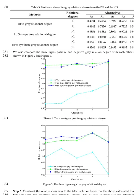
Table 3. Positive and negative grey relational degree from the PIS and the NIS
380
Methods Relational
degrees
Alternatives
A1 A2 A3 A4 A5
HFSs grey relational degree
w
γ+
0.4934 0.4984 0.5922 0.6250 0.6949
w
γ−
0.6942 0.7630 0.6867 0.7325 0.5583
HFSs slope grey relational degree
sw
γ+
0.8854 0.8882 0.8901 0.9021 0.9107
sw
γ−
0.8086 0.8288 0.8265 0.8929 0.8188
HFSs synthetic grey relational degree
cw
γ+
0.8640 0.8676 0.9054 0.8658 0.9251
cw
γ−
0.8366 0.8605 0.8493 0.8883 0.8160 We also compare the three types positive and negative grey relation degree with each other as
381
shown in Figure 2 and Figure 3.
382
1 2 3 4 5
0.45 0.5 0.55 0.6 0.65 0.7 0.75 0.8 0.85 0.9 0.95
Alternatives
R
el
at
iv
e cl
os
en
es
s
HFSs positive grey relative degree HFSs slope positive grey relative degree HFSs synthetic positive grey relative degree
Figure 2. The three types positive grey relational degree
383
1 2 3 4 5
0.55 0.6 0.65 0.7 0.75 0.8 0.85 0.9 0.95
Alternatives
R
ela
ti
ve
c
lo
se
ne
ss
HFSs negative grey relative degree HFSs slope negative grey relative degree HFSs synthetic negative grey relative degree
Figure 3. The three types negative grey relational degree
384
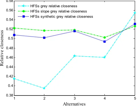
Step 3: Construct the relative closeness to the ideal solution based on the above calculated three
385
( 1, 2, , ) i
A i= m with respect to the ideal solution are shown as Table 4 and the compared effect of
387
the three methods is shown in Figure 4.
388
Table 4. The three types grey relative closeness of the 5 alternatives to the ideal solution
389
Relative closeness Alternatives Rankings
A1 A2 A3 A4 A5
HFSs grey relative closeness 0.4155 0.3951 0.4631 0.4604 0.5545 A5A3A4A1A2 HFSs slope grey relative
closeness 0.5227 0.5173 0.5185 0.5026 0.5266 A5A1A3A2 A4 HFSs synthetic grey relative
closeness 0.5081 0.5020 0.5160 0.4936 0.5313 A5A3A1A2 A4 Step 4: Rank the alternatives according to the decreasing order of the three types relative closeness,
390
shown as Table 4 too.
391
Consequently, we select the best one with the greatest relative closeness to the ideal solution
392
and all the three types relative closeness indicate that the decision result is alternative A5.
393
Compared the decision results, we can see that the decision result is consistent with the decision
394
result from reference [7, 10, 12, 18, 52, 53], which derived from different distance and similarity
395
measures. It proves that the three types grey relation methods are effective in the hesitant fuzzy
396
decision problems, successfully apply the grey relation analysis theory into the hesitant fuzzy
397
domain.
398
1 2 3 4 5
0.38 0.4 0.42 0.44 0.46 0.48 0.5 0.52 0.54 0.56 0.58
Alternatives
R
el
at
ive cl
osenes
s
HFSs grey relative closeness HFSs slope grey relative closeness HFSs synthetic grey relative closeness
Figure 4. The three types relative closeness
399
5.2. Apply the proposed grey relational based MADM methodology to emergency management evaluation
400
example
401
In this section, followed by the MADM example with interval-valued hesitant fuzzy
402
information concerning emergency management evaluation problems, these data are extracted from
403
Reference [34].
404
Suppose that there are four alternatives A ii( =1, 2,3, 4) to be evaluated by evaluators, each
405
alternative has these six attributes C ii( =1, 2, ,6) , and assume the attribute weight is known, let the
406
weight w=(0.1074, 0.1205,0.2101,0.1428, 0.2474,0.1718)T . The evaluated values are expressed by
407
interval-valued hesitant fuzzy information in an interval-valued hesitant fuzzy decision matrix,
408
shown in Table5.
409
Table 5. The Interval-valued hesitant fuzzy attributes information
411
Attribute Alternatives
A1 A2 A3 A4
Attribute1 {[0.7,0.9],[0.7,0.8],[0.6,0.8]} {[0.5,0.7],[0.5,0.6],[0.4,0.6]} {[0.3,0.5],[0.2,0.4],[0.2,0.3]} {[0.6,0.7],[0.5,0.7],[0.5,0.6]} Attribute2 {[0.4,0.5],[0.2,0.3],[0.1,0.3]} {[0.5,0.7],[0.5,0.5],[0.4,0.5]} {[0.8,0.9],[0.7,0.8],[0.6,0.8]} {[0.4,0.6],[0.3,0.6],[0.3,0.4]} Attribute3 {[0.2,0.4],[0.2,0.3],[0.1,0.3]} {[0.8,1.0],[0.7,0.9],[0.6,0.8]} {[0.3,0.4],[0.2,0.4],[0.1,0.4]} {[0.3,0.5],[0.2,0.4],[0.2,0.3]} Attribute4 {[0.5,0.8],[0.4,0.7],[0.4,0.6]} {[0.9,1.0],[0.7,0.9],[0.6,0.8]} {[0.2,0.3],[0.1,0.3],[0.1,0.2]} {[0.3,0.5],[0.3,0.4],[0.2,0.4]} Attribute5 {[0.2,0.5],[0.2,0.4],[0.1,0.4]} {[0.8,0.9],[0.7,0.9],[0.7,0.8]} {[0.1,0.3],[0.0,0.2],[0.0,0.1]} {[0.1,0.2],[0.0,0.2],[0.0,0.1]} Attribute6 {[0.8,0.9],[0.7,0.8],[0.7,0.7]} {[0.9,1.0],[0.8,1.0],[0.8,0.9]} {[0.6,0.8],[0.6,0.7],[0.5,0.5]} {[0.6,0.7],[0.4,0.6],[0.4,0.5]}
We utilize the proposed grey relational based MADM methodology to evaluate the alternatives
412
with IVHFSs information in the following steps:
413
Step 1: All the attribute are benefit type, we select each maximum IVHFE in the five alternatives
414
IVHFSs on the four attribute to construct the interval-valued hesitant fuzzy PIS A+ and each
415
minimum IVHFE to construct the interval-valued hesitant fuzzy the NIS A−:
416
[
] [
] [
]
{
}
{
[
] [
] [
]
}
{
[
] [
] [
]
}
[
] [
] [
]
{
}
{
[
] [
] [
]
}
{
[
] [
] [
]
}
+=[ 0.7,0.9 , 0.7,0.8 , 0.6,0.8 , 0.8,0.9 , 0.7,0.8 , 0.6,0.8 , 0.8,1.0 , 0.7, 0.9 , 0.6, 0.8 ,
0.9,1.0 , 0.7, 0.9 , 0.6, 0.8 , 0.8,0.9 , 0.7,0.9 , 0.7,0.8 , 0.9,1.0 , 0.8,1.0 , 0.8,0.9 ] A
,
417
[
] [
] [
]
{
}
{
[
] [
] [
]
}
{
[
] [
] [
]
}
[
] [
] [
]
{
}
{
[
] [
] [
]
}
{
[
] [
] [
]
}
=[ 0.3,0.5 , 0.2,0.4 , 0.2,0.3 , 0.4, 0.5 , 0.2,0.3 , 0.1,0.3 , 0.2,0.4 , 0.2,0.3 , 0.1,0.3 , 0.2, 0.3 , 0.1,0.3 , 0.1,0.2 , 0.1,0.2 , 0.0,0.2 , 0.0,0.1 , 0.6,0.7 , 0.4,0.6 , 0.4,0.5 ] A−418
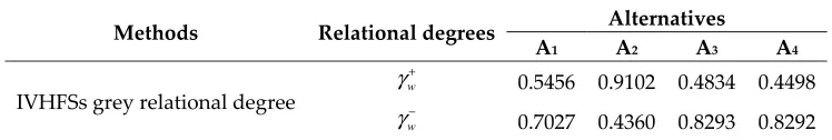
Step 2: Calculate the IVHFSs positive and negative grey relational degrees between each alternative
419
and the PIS and NIS, respectively. We assume the distinguished coefficient ρ =0.5. The result is
420
shown as Table 6.
421
Table 6. IVHFSs positive and negative grey relational degree from the PIS and the NIS
422
Methods Relational degrees Alternatives
A1 A2 A3 A4
IVHFSs grey relational degree
w
γ+
0.5456 0.9102 0.4834 0.4498
w
γ−
0.7027 0.4360 0.8293 0.8292
Step 3: Construct the relative closeness to the ideal solution based on the calculated IVHFSs positive
423
and negative grey relational degree. The IVHFSs relative closeness of the alternative A ii( =1, 2,3, 4)
424
are shown as Table 7.
425
Table 7. The IVHFSs relative closeness of the 4 alternatives to the ideal solution
426
Relative closeness Alternatives Rankings
A1 A2 A3 A4
IVHFSs grey relative closeness 0.4371 0.6761 0.3683 0.3517 A2A1A3A4
Step 4: Rank the alternatives according to the decreasing order of The IVHFSs relative closeness also
427
shown in Table 7.
428
It can be clearly seen from Table 7 that the decision result is the alternative A2. It is consistent
429
with the decision result from reference [34], which illustrates the validity and accuracy of the
430
proposed IVHFSs grey relational MADM methodology.
431
Combined with two practical MADM examples about energy policy selection with HFSs
432
information and emergency management evaluation with IVHFSs information, we can see that the
433
proposed grey relational based MADM methodology can deal with the HFSs and IVHFSs MADM
434
demonstrates the grey relational based MADM methodology’s effectiveness. Furthermore, it is the
436
first time to apply the grey relational analysis theory to the HFSs and IVHFSs field, which greatly
437
enrich the fuzzy measures of HFSs and is significant in the development of the HFSs.
438
6. Conclusions
439
In this paper, we apply the grey relational analysis theory to the HFSs and IVHFSs domain and
440
propose three types grey relational degree: the HFSs grey relational degree, HFSs slope grey
441
relational degree and HFSs synthetic grey relational degree, which describe the closeness, the
442
variation tendency and both the closeness and variation tendency of the HFSs, respectively. We also
443
propose the grey relational degree for the IVHFSs. We deduce these grey relational degrees for HFSs
444
and IVHFSs in detail. Additionally, we develop the HFSs grey relational based MADM
445
methodology based on the TOPSIS method to solve the HFSs and IVHFSs MADM problems. Finally,
446
combined with two practical MADM examples about energy policy selection with HFSs information
447
and emergency management evaluation with IVHFSs information, we obtain the appropriate
448
decision results. Compared with the decision results with the previous methods, it illustrates the
449
validity, effectiveness and accuracy of the proposed grey relational based MADM methodology.
450
In the future, we will apply the proposed grey relational analysis methodology for HFSs and
451
IVHFSs to some other fields as pattern recognition and deep learning. Also, we will attempt to apply
452
the grey analysis theory to the Dual hesitant fuzzy sets and hesitant fuzzy linguistic sets.
453
Acknowledgments: This work is supported by the Major Research Plan of the National Natural Science
454
Foundation of China (Grant no. 91538201), the National Natural Science Foundation of China (Grant nos.
455
61671463, 61571454), the Natural Science Foundation of Shandong Province (Grant no. ZR2017BG014) and the
456
Program for New Century Excellent Talents in University(Grant no. NCET-11-0872).
457
Author Contributions: In this paper, the idea and primary algorithm were proposed by Guidong Sun. Xin
458
Guan refined the idea and solution models. Xiao Yi and Jing Zhao conducted the simulation and analysis of
459
the paper.
460
Conflicts of Interest: The authors declare no conflict of interest.
461
References
462
463
1. Torra V. Hesitant fuzzy sets. International Journal of Intelligent Systems, 2010, 25, 529-539.
464
2. Torra V.; Narukawa Y. On hesitant fuzzy sets and decision. The 18thIEEE International Conference on
465
Fuzzy Systems, Jeju Island, Korea, 2009, 1378-1382.
466
3. Xia M.M.; Xu Z.S. Hesitant fuzzy information aggregation in decision making. International Journal of
467
Approximate Reasoning, 2011, 52 (3), 395-407.
468
4. Xia M.M.; Xu Z.S.; Chen N. Some hesitant fuzzy aggregation operators with their application in group
469
decision making. Group Decision and Negotiation, 2013, 22, 259-279.
470
5. Liao H.C.; Xu Z.S. Subtraction and division operations over hesitant fuzzy sets. Journal of Intelligent &
471
Fuzzy Systems, 2014, 27 (1), 65-72.
472
6. Liao H.C.; Xu Z.S.; Xia M.M. Multiplicative consistency of hesitant fuzzy preference relation and its
473
application in group decision making. International Journal of Information Technology & Decision
474
Making, 2014, 13 (1), 47-76.
475
7. Xu Z.S.; Xia M.M. Distance and similarity measures for hesitant fuzzy sets. Information Sciences, 2011,181,
476
2128-2138
477
8. Xu Z.S.; Xia M.M. On distance and correlation measures of hesitant fuzzy information. International
478
Journal of Intelligent Systems, 2011, 26, 410-425.
479
9. Xu Z.S.; Xia M.M. Hesitant fuzzy entropy and cross-entropy and their use in multiattribute
480
decision-making. International Journal of Intelligent Systems. 2012, 27, 799-822.
481
10. Farhadinia B. Distance and similarity measures for higher order hesitant fuzzy sets. Knowledge-Based
482
Systems, 2014, 55, 43-48.
483
11. Farhadinia B. Information measures for hesitant fuzzy sets and interval-valued hesitant fuzzy sets.