Non-linear Indeterminate Equations
(Giophantus)
Koichiro Akiyama1, Yasuhiro Goto2, Shinya Okumura3⋆, Tsuyoshi Takagi4, Koji Nuida5, Goichiro Hanaoka5, Hideo Shimizu1, and Yasuhiko Ikematsu4
1 Corporate Research& Development Center, Toshiba Corporation {koichiro.akiyama,hideo.shimizu}@toshiba.co.jp
2 Department of Mathematics, Hokkaido University of Education at Hakodate
3 Department of Information and Communications Technology, Osaka University
4
Institute of Mathematics for Industry, Kyushu University
{takagi,y-ikematsu}@imi.kyushu-u.ac.jp
5
National Institute of Advanced Industrial Science and Technology
{k.nuida,hanaoka-goichiro}@aist.go.jp
Abstract. In this paper, we propose a post-quantum public-key en-cryption scheme whose security depends on a problem arising from a multivariate non-linear indeterminate equation. The security of lattice cryptosystems, which are considered to be the most promising candidate for a post-quantum cryptosystem, is based on the shortest vector prob-lem or the closest vector probprob-lem in the discrete linear solution spaces of simultaneous equations. However, several improved attacks for the underlying problems have recently been developed by using approxima-tion methods, which result in requiring longer key sizes. As a scheme to avoid such attacks, we propose a public-key encryption scheme based on the “smallest” solution problem in thenon-linear solution spaces of multivariateindeterminate equations that was developed from the alge-braic surface cryptosystem. Since no efficient algorithm to find such a smallest solution is currently known, we introduce a new computational assumption under which proposed scheme is proven to be secure in the sense of IND-CPA. Then, we perform computational experiments based on known attack methods and evaluate that the key size of our scheme under the linear condition. This paper is a revised version of [4].
Keywords:Public-key Cryptosystem, Post-Quantum Cryptosystem, Inde-terminate Equation, Smallest Solution Problem
⋆
1
Introduction
In 1994, Shor proposed quantum algorithms that can solve the factorization problem and the discrete logarithm problem in polynomial time [47]. This im-plies that elliptic curve cryptosystems and the RSA cryptosystem will no longer be secure once a quantum computer is built. Due to this, the importance of “Post-quantum cryptosystems” (PQCs) that will still be secure after the de-velopment of quantum computers has been recognized. With the recent active studies to develop quantum computers, NIST announced that the process of PQC standardization will begin in the end of 2017 [40]. Possible candidates for a PQC include lattice-based encryptions, code-based encryptions, and multivari-ate encryptions.
First lattice-based encryption was proposed in 1997 by Ajtai and Dwork [1]. Its security depends on the unique shortest vector problem in lattices. Goldreich et al. proposed the GGH cryptosystem, whose security is based on the closest vec-tor problem for an integer lattice [24]. However, according to Nguyen and Stern, these schemes are not practical since they require large size parameters for se-curity reasons [36, 35]. Hoffstein et al. proposed the NTRU cryptosystem, whose security depends on the shortest vector problem for polynomial ring lattices [25]. In 2009, Regev proposed an LWE cryptosystem, whose security depends on the “learning with error” (LWE) problem [45]. Currently, NTRU, LWE, and their variants are relatively efficient among lattice-based encryption schemes.
However, there are several efficient approximation algorithms for finding the (nearly) shortest/closest vectors, such as the LLL [30], BKZ [46], and BKZ2.0 [15] algorithms. Recently, several improved attacks for these underlying problems using these methods, such as lattice decoding attacks [10] and subfield lattice attacks [28] have been developed. In order to avoid these attacks, the public-key sizes of lattice-based cryptosystems must be enlarged. Encryption schemes with large key sizes require a large amount of memory in applications.
Code-based encryption was first proposed in 1978 by McEliece [33]. Its secu-rity depends on the decoding problem for random linear codes, for which only exponential algorithms are known. However, it requires a large public-key size, of more than 1M bits. The multivariate public-key cryptosystem (MPKC) was first introduced in 1989 by Matsumoto and Imai [26] and was improved by Patarin [43]. Its security depends on the problem of solving non-linear equations (called multivariate equations) over finite fields. While the problem is NP-hard in gen-eral, almost all proposed schemes have been broken due to the special structure of the equations that are used as public keys. Several schemes with resistance against known attacks on MPKC have been proposed, but they still have large public keys [44, 49, 53].
proposed the algebraic surface cryptosystem (ASC) [3], whose security depends on the section-finding problem (the problem of solving some kind of indetermi-nate equation). Although they claimed that their proposed scheme necessitates much shorter public keys than the other candidates for PQC, the scheme was broken by Faug´ere et al. [19]. In this paper, we intend to improve ASC by modifying the underlying problem to make the scheme secure while keeping the public-key size small relative to that of other PQC candidates.
Our Contribution. This paper proposes a post-quantum public-key encryption scheme whose security is based on the smallest solution problem for non-linear solution spaces of indeterminate equations, to which attack algorithms based on approximation (e.g., LLL and BKZ) cannot be applied. Our scheme was developed from ASC, which is designed such that its security depends on the intractability of solving some non-linear indeterminate equation [3]. ASC was broken by the ideal decomposition attack proposed in PKC 2010 [19]. We revise the scheme to be secure against this attack by adding a noise term to the cipher polynomial. Our scheme is provably secure in the sense of IND-CPA under the intermediate equation of LWE (IE-LWE) assumption, which is a new computa-tional assumption coming from analogy to the LWE assumption. An IND-CCA2 secure scheme is obtained by using a well-known conversion technique [20].
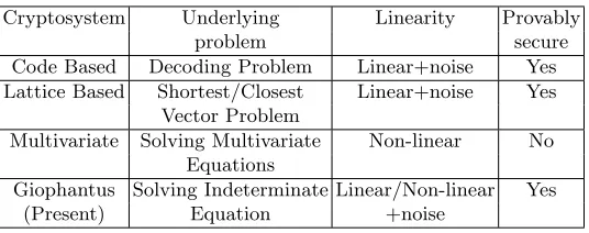
We refer to the public key encryption scheme as theGiophantusTM encryp-tion scheme, which comes from the Diophantine equaencryp-tions used as the general term for the indeterminate equations in integers6. In addition, the Giophantus encryption scheme has the ring homomorphic property described in Section 11. Table 1 shows the difference between Giophantus and other post-quantum cryptography (PQC) candidates. In Table 1, “Linearity” indicates the linearity of the underlying problem. Giophantus provides public-key cryptosystem whose security depends on the computational hardness of solving indeterminate equa-tions. Solving non-linear indeterminate equations is a well-known hard problem in general. In particular, it is known that there is no general solution for equations overZorFq[t] and no general algorithm for solving them. Although this encryp-tion scheme employs indeterminate equaencryp-tions over Fq[t]/(tn−1), the scheme itself is potentially secure since we are able to apply non-linear equations to the scheme.
This paper is organized as follows. Section 2 gives our notation and the section 3 introduces basic mathematical definitions. In the section 4, we re-call the algebraic surface encryptions, which our scheme was developed from. In section 5, we define domain parameters and propose our encryption primi-tive. Section 6 provides the computational assumption that makes our scheme provably secure. In the section 7, we discuss some considerable attacks against this assumption with computational experiments and the section 8 provides
ap-6
Table 1.Comparison with other PQC candidates
Cryptosystem Underlying Linearity Provably
problem secure
Code Based Decoding Problem Linear+noise Yes Lattice Based Shortest/Closest Linear+noise Yes
Vector Problem
Multivariate Solving Multivariate Non-linear No Equations
Giophantus Solving Indeterminate Linear/Non-linear Yes
(Present) Equation +noise
propriate parameters. The section 9 makes our primitive IND-CCA secure by applying Fujisaki-Okamoto conversion and the section 10 shows performance of our scheme. The section 11 shows that our IND-CPA primitive has homomorphic properties which will be benefit to cloud computing. We summarize the results and discuss directions for future work in Section 12.
2
Notation
The notation in this paper includes the following.
M Plaintext in the set {0,1}k, wherekis bit length of the plaintexts. The bit length is defined in domain parameters which is described in Section 5.1.
ℓ A small integer which is larger than 1
(m1m2· · ·mk)ℓ ℓ-ary representation of plaintextM, particularly the caseℓ= 2, which is binary representation.
q A prime number much larger thanℓ
Fq The prime field identified with the set{0,· · · , q−1}
x, y, t Variables used for the cryptographic primitives and
scheme
Fq[t] Univariate polynomial ring overFq
Rq Quotient ring Fq[t]/(tn−1), which is Fq[t] modulo
tn−1, wherenis an integer larger than 1
Rℓ Subset of the quotient ringRq, which consists of all univariate polynomials oftup to degreen−1 whose coefficients are within the range{0,· · ·, ℓ−1}
Z[t]/(tn−1) Quotient ring, which is Z[t] modulo tn−1 where n
is an integer larger than 1
n Degree of the modulustn−1 of the quotient ringR q
max(S) Maximum value of ordered set S. If S =
{3,8,−3,4,9}, then max(S) = 9.
X(x, y) Irreducible bivariate polynomial ofxandy over the ringRq, withX(x, y) an element ofRq[x, y]
r(x, y) Random bivariate polynomial of x and y over the ringRq, withr(x, y) an element ofRq[x, y]
e(x, y) Noise bivariate polynomial of xandy over the ring
Rq, withe(x, y) an element ofRℓ[x, y]
m(t) Plaintext polynomial that embeds a plaintextM into
Rℓ
c(x, y) Ciphertext polynomial over the ring Rq such that
c(x, y) is an element ofRq[x, y]
(ux(t), uy(t)) Small solution of the indeterminate equation
X(x, y) = 0 over the ring Rq, whereux(t) anduy(t) are polynomials of t in Rℓ and satisfy the relation
X(ux(t), uy(t)) = 0
aij(t) Coefficient of the monomial xiyj belonging to the irreducible bivariate polynomialX(x, y) over the ring
Rq, such thataij(t) is an element ofRq
rij(t) Coefficient of the monomial xiyj belonging to the random bivariate polynomialr(x, y) over the ringRq, such thatrij(t) is an element ofRq
eij(t) Coefficient of the monomial xiyj belonging to the noise bivariate polynomial e(x, y) over the set Rℓ, such thateij(t) is an element ofRℓ
ΓX Support set of the irreducible polynomial X(x, y). Each element is a pair (i, j) of the exponents ofxiyj, which is a non-zero monomial ofX(x, y) such that
ΓX ={(i, j)∈(N∪ {0})2|aij(t)̸= 0}. #ΓX Cardinality of the support setΓX
FΓX/Rq Set of bivariate polynomials whose support set isΓX over the ringRq
Γr Support set of the random polynomialr(x, y). Each element is a pair (i, j) of the exponents of a non-trivial monomialxiyj.
#Γr Cardinality of the support setΓr
FΓr/Rq Set of bivariate polynomials whose support set isΓr over the ringRq
Γe Support set of the random polynomiale(x, y). Each element is a pair (i, j) of the exponents of a non-trivial monomialxiyj.
#Γe Cardinality of the support setΓe
FΓe/Rℓ Set of bivariate polynomials whose support set isΓe over the ringRℓ
X(ΓX, ℓ)/Rq Subset ofFΓX/Rq, consisting of all bivariate polyno-mials with a small zero point (ux(t), uy(t)) inRℓ
dX Total degree of irreducible bivariate polynomial
X(x, y) such that
dX=max({i+j|X(x, y) =∑(i,j)∈Γ
Xaij(t)x iyj })
dr Total degree of random bivariate polynomialr(x, y) such that
dr=max({i+j |r(x, y) =∑(i,j)∈Γ
rrij(t)x iyj }) |.| Bit length of an integer, such as|5|= 3
3
Preliminaries
In this section, we introduce some basic mathematical definitions and operations needed in this paper.
3.1 Finite fields and polynomial Rings
A field is defined as a set with operations such as addition, subtraction, multipli-cation and division that satisfy certain rules. Typical examples of fields are the real number fieldR, the rational number fieldQand finite fieldsFq. Finite fields
Fq are fields with q elements, whereq is a positive integer, called the order. It is well known that the order is a primepor a prime powerpk. A prime field is defined as a finite field whose order is prime. In this paper, we focus on the case of prime fields written as sets:
Fq ={0,1,· · · , q−1}.
Its operations are described using the modulus ofqas follows:
a+b=a+b modq, a−b=a−b modq, a·b =a·b modq, a/b =a·b−1 modq,
(1)
whereb−1 satisfies the conditionb·b−1= 1 modq.
Example 1. The prime field F5={0,1,2,3,4} can be equipped with operations modulo 5, such as
1 + 2 = 3, 2 + 4 = 1, 3−1 = 2, 2−3 = 4,
2·2 = 4, 2·3 = 1, 2/3 = 2·3−1= 2·2 = 4.
LetR be a ring. A univariate polynomial ring is a set defined as
R[t] ={c0+c1t+· · ·+cntn |ci ∈R(0≤i≤n)n∈N}, (2) where t is a variable and ci is the coefficient of the monomial citi. Univariate polynomialsf(t) andg(t) can be described as
f(t) =a0+a1t+· · ·+antn,
g(t) =b0+b1t+· · ·+bntn,
(3)
where ai andbi are elements of R. We note that neitheran = 0 norbn = 0 is assumed in the expression of (3) above.
R[t] is a ring since addition and multiplication are defined as follows:
f+g=a0+b0+ (a1+b1)t+· · ·+ (an+bn)tn,
f·g =a0·b0+ (a1·b0+a0·b1)t+· · ·+ (an·bn)t2n.
Though an inverse of addition can be defined as −f =−a0−a1t− · · · −antn,
an inverse of multiplication can be defined if and only if f(t) is a non-zero constant, such as f(t) =a0.
Example 2. Let us consider a univariate polynomial in F5[t] and set f(t) = 2 + 3t+ 4t2andg(t) = 4 +t+ 3t2. Then,f(t) +g(t) = 1 + 4t+ 2t2,f(t)·g(t) = 2t4+ 3t3+ 4t+ 3, and−f(t) = 3 + 2t+t2.
F5[t] ={c0+c1t+· · ·+cntn |ci∈F5(0≤i≤n)n∈N} . (5) If a polynomial is written inf(t) =∑ni=0citisuch that the coefficientcn ̸= 0 then we define nto be the degree of f. Thus, the degree off is the maximum integernsuch thatcn̸= 0. We denote this by degf =n. In the example off(t) andg(t) above,
deg(f) = deg(g) = 2, deg(f(t)·g(t)) = 4.
A bivariate polynomial ring is a set defined as
R[x, y] ={cn0xn+c(n−1)1xn−1y+· · ·+c0nyn+· · ·+c10x+c01y+c00 |cij∈R(0≤i, j≤n)n∈N},
(6)
wherexandy are variables andcij are coefficients of the monomialcijxiyj. Setf(x, y) andg(x, y) as follows:
f(x, y) =∑ni=j=1aijxiyj
=an0xn+a(n−1)1xn−1y+· · ·+a0nyn+· · ·+a10x+a01y+a00,
g(x, y) =∑ni=j=1bijxiyj
=bn0xn+b(n−1)1xn−1y+· · ·+b0nyn+· · ·+b10x+b01y+b00, (7)
whereaij andbij are elements ofR. Then we define addition and multiplication as follows:
f+g=∑ni=j=0(aij+bij)xiyj
= (an0+bn0)xn+ (a(n−1)1+b(n−1)1)xn−1y+· · ·+ (a10+b10)x +(a01+b01)y+a00+b00,
f·g =∑ni
1+j1=i2+j2=0(ai1j1bi2j2)x
iyj
= (an0bn0)x2n+ (an0b(n−1)1+a(n−1)1bn0)x2n−1y+· · · +(a01b00+a00b01)y+a00b00.
(8)
An inverse of addition can be defined as
Example 3. In the case of F5[x, y], set
f(x, y) = 2x2+ 3xy+y2+ 3x+ 3y+ 4,
g(x, y) =x2+ 2xy+ 3y2+x+ 3y+ 3, (9) and thenf(x, y) +g(x, y) = 3x2+ 4y2+ 4x+y+ 2,
f(x, y)·g(x, y) = 2x4+ 2x3y+ 3x2y2+xy3+ 3y4+ 3x2y+ 2y3+ 3x2 +4xy+ 4y2+ 3x+y+ 2
and−f(x, y) = 3x2+ 2xy+ 4y2+ 2x+ 2y+ 1.
Setting the bivariate polynomialf(x, y) =∑ni=j=0cijxiyj, the total degree off, denoted degf, can be defined as
degf :=max({i+j|cij̸= 0}).
We can determine the degrees forf(x, y) andg(x, y), described above, as follows. deg(f(x, y)) = deg(g(x, y)) = 2, deg(f(x, y)·g(x, y)) = 4.
3.2 The quotient ring Rq
The ringRq is defined as the quotient ring ofFq[t] modulotn−1. Elements of
Rq are polynomials overFq with degree at mostn−1 (sincetn is equivalent to 1).
We can representa∈Rq as a vector (a0, a1,· · · , an−2, an−1) representing
a=a0+a1t+· · ·+an−2tn−2+an−1tn−1
on Fq. When elements b, c∈ Rq are represented in the same manner as a, we can expressab+c as
(
b0b1· · ·bn−2bn−1 )
a0 a1 · · ·an−2an−1 an−1 a0 · · ·an−3an−2 an−2an−1· · ·an−4an−3
..
. ... ... ... ...
a1 an−1· · ·an−1 a0
+(c0c1· · ·cn−2cn−1 )
(10)
onFq.
Using this expression, the relationab+c=dcan be described as
bA+c=d,
3.3 Monomial order
To describe a detailed specification of the proposal, we need to introduce the monomial order of polynomials, which defines the order of calculation. First, we define an exponent vector α= (i, j)∈Z2≥0 of monomialxiyj, and then we denote a monomialxiyj as xα.
Example 4. The exponent vectors of monomials 3x2y3 and 4x3 in Fq[x, y] are (2,3) and (3,0) respectively.
We define the monomial orderingxα> xβ as follows.
Definition 1. A monomial ordering on bivariate polynomial ringFq[x, y]is any
relation >on the set of monomials inFq[x, y] orZ2
≥0 satisfying:
1. > is a total ordering such that any pair of monomials α and β satisfies exactly one of the relationsα < β,α=β, andα > β.
2. >is compatible with multiplication in Fq[x, y]. If α > β and there is some
γ∈Z2≥0 thenα+γ > β+γ since the relationxαxγ > xβxγ is satisfied. 3. > induces a well ordering, such that there is a minimum element in any
non-empty subset ofZ2≥0 or monomial set.
Lexicographic ordering is an example of monomial ordering satisfying these rules. It is defined as follows.
Definition 2. For any α = (α1, α2)∈ Z2≥0 and β = (β1, β2) ∈Z2≥0, the
rela-tion α >lex β (resp., α <lex β) holds when the leftmost non-zero entry of the
difference of the exponent vectors α−β is positive (resp., negative). We write xα>
lexxβ if α >lexβ and analogously for<lex.
For example, (2,1) >lex (1,2) since the difference of the exponent vectors
α−β = (1,−1). Similarly, (2,1) <lex (2,2) since α−β = (0,−1), and the leftmost non-zero entry is negative.
In this paper, we employ the graded lexicographic order, which is defined as follows.
Definition 3. Let xα andxβ be monomials inFq[x, y]. We definexα<grlexxβ
ifα1+α2> β1+β2, or ifα1+α2=β1+β2 and in the difference vectorα−β,
the leftmost non-zero entry is positive.
For example, we have (0,2)>grlex(1,0) sinceα1+α2= 2>1 =β1+β2. In the case of (1,1)>grlex(0,2), we haveα1+α2= 2 =β1+β2andα−β= (1,−1), the leftmost non-zero entry is positive.
3.4 Support set of a polynomial
Let’s R be a set. Let’s X(x, y) be a bivariate polynomial over R written as
∑
(i,j)∈(N∪{0})2aijxiyj, whereaij is an element ofR. Then we can define a sup-port set of a polynomialX(x, y) over the setR as
ΓX={(i, j)∈(N∪ {0})2|aij̸= 0s.t. X(x, y) =
∑
(i,j)∈(N∪{0})2
The support setΓX specifies the monomials which belongs to a bivariate poly-nomialX(x, y). In addition, we can define the support setΓXrfor given support setsΓX andΓr as follows.
ΓXr=
{(i, j)∈(N∪ {0})2|i=i1+i2, j=j1+j2s.t.(i1, j1)∈ΓX,(i2, j2)∈Γr} (11) TheΓXris a support set of the polynomialXr’s, whereX andrare polynomials whose support sets areΓX andΓrrespectively.
The bivariate polynomial set of all polynomials whose support set is a subset ofΓX is defined as
FΓX/R={f(x, y)∈R[x, y]|aij ̸= 0⇒(i, j)∈ΓX} . (12)
4
Design concept
4.1 Algebraic Surface Cryptosystem
The ASC was first announced in 2006 by K. Akiyama and Y. Goto [2]. The algebraic surfaces are defined as a solution space of a three-variable polynomial equation X(x, y, t) = 0 over a field K. The security of ASC depends on the section-finding problem, defined as follows.
Definition 4. (Section-finding problem) IfX(x, y, t) = 0 is an algebraic surface over a fieldK, then the problem of finding a parameterized curve
(x, y, t) = (ux(t), uy(t), t) onX is called thesection-finding problem onX. A section can be considered as a solution ofX(x, y) = 0, which is an inde-terminate equation over the ringK[t].
The problem of solving indeterminate equations over an arbitrary ring or field is known to be hard. For example, the class of indeterminate equations over the integer ring Z, called Diophantine equations, is undecidable (Hilbert’s 10th problem). Being “undecidable” means that there is no general algorithm to solve such indeterminate equations. The section-finding problem has been proven to be undecidable [17].
We recall the method of algebraic surface encryption to see the conceptual design for the scheme described in this paper. First, the simplest ASC can be described as
c(x, y) =m(x, y) +X(x, y)r(x, y),
whereX(x, y) is the public key, which defines an algebraic surface with a section. The polynomials c(x, y) and r(x, y) are a ciphertext polynomial and a random polynomial, respectively. The polynomial m(x, y) is a plaintext polynomial in which a plaintext message is embedded. In the decryption phase, we substitute the secret key (a section ofX(x, y)) intoc(x, y). By the relationX(ux(t), uy(t)) = 0, we obtain
From the polynomial m(ux(t), uy(t)), we can recover the plaintext message as follows. We can describem(x, y) as
m(x, y) = ∑ (i,j,k)∈Γm
mijkxiyjtk,
where each mijk is a variable, and substitute the section intom(x, y). We thus obtain
m(ux(t), uy(t)) =
∑
(i,j,k)∈Γm
mijkux(t)iuy(t)jtk.
Comparing the coefficient oft, the simultaneous linear equations containingmijk are constructed. When the number of variables is less than or equal to the number of equations, we can detect the correct plaintext message by solving the equations.
However, there exists an attack to break the scheme. We can expand the cipher polynomialc(x, y) to
c(x, y) = ∑ (i,j,k)∈Γm
mijkxiyjtk+
∑
(i,j,k)∈ΓX
aijkxiyjtk
∑
(i,j,k)∈Γr
rijkxiyjtk
,
(13) whereΓm,ΓX, andΓrare given as parameters, and the valuesaijk are the given coefficients of the public key X. Each mijk and rijk is a variable. Comparing the coefficients of the monomials, we obtain the simultaneous linear equations having the variablesmijk andrijk. For decryption, the relation
#Γm+ #Γr<#ΓXr
is required. However, in this case, the equations have unique solution with high probability. We refer to this type of attack as the Linear Algebra attack.
To avoid the attack, K. Akiyama, Y. Goto and H. Miyake constructed the lat-est ASC scheme in 2009 [3]. From the cryptographic point of view, the ciphertext is equivalent to
c(x, y) =m(x, y)s(x, y) +X(x, y)r(x, y). (14) Here, s(x, y) is employed as another random polynomial and the term product
m(x, y)s(x, y) equals X(x, y)r(x, y) (with Γms =ΓXr). To decrypt the cipher-text, we have to divide m(ux(t), uy(t))s(ux(t), uy(t)) into m(ux(t), uy(t)) and
s(ux(t), uy(t)) by factoring. Since polynomial factoring is computationally easy via the Berlekamp method, we can obtainm(ux(t), uy(t)) as a factor. The plain-text is then recovered from m(ux(t), uy(t)) in the same way as in the previous scheme.
Applying the Linear Algebra attack to this scheme, we need to consider
#Γr+ #ΓXr, is greater than the number of equations, #ΓXr, and so the Linear Algebra attack does not work.
Unfortunately, this scheme was also broken by the ideal decomposition attack, which was described by Faugere et al. [19]. They found that the ideal (c(x, y), X(x, y)) can be decomposed into (m(x, y), X(x, y)) and (s(x, y), X(x, y)) by calculating the resultant Resx(c(x, y), X(x, y)) and Resy(c(x, y), X(x, y)). The plaintext messagem(x, y) is then recovered by solving the linear equations. The proposed primitive avoids both attacks. Our idea is to apply for the
ℓ-polynomial structure employed in NTRU encryption. The ciphertext is
c(x, y) =m(x, y) +X(x, y)r(x, y) +ℓ·e(x, y),
where e(x, y) is a random polynomial whose coefficients are small. The polyno-miale(x, y) works as a noise factor in the cipher, and we claim the condition
#Γe= #ΓXr
for resistance against the Linear Algebra attack. Needing the smallest solution ofX(x, y) to decrypt the message ensures this.
5
Our Proposed Encryption Scheme
This section provides an overview of the proposed encryption scheme.
5.1 Domain parameters
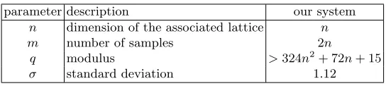
We introduce parameters for the proposed scheme to be input to the key gener-ation algorithm. Appropriate parameter settings are discussed in Section 8.
– ℓ: A small integer which is larger than 1.
– q: A prime which is cardinality of prime fieldFq and is much larger than
ℓ.
– n: Degree of the modulus polynomial of the quotient ringRq(=Fq[t]/(tn− 1)). Thenshould be prime for the security reason.
– dX: Total degree of the irreducible bivariate polynomialX(x, y) – dr: Total degree of the random bivariate polynomialr(x, y) – mlen Length of the messageM
The relation between ℓ and qis a critical condition for decryption. We require the condition
q > ℓ−1 +ℓ
dX∑+dr
k=0
(k+ 1)nk(ℓ−1)k+1 (15)
to decrypt any ciphertext encrypted by the proposed encryption primitive. The support set of the irreducible polynomialX(x, y) with total degreedX
is defined such that
with graded lexicographic order. If dX is equal to 2, then
ΓX ={(2,0),(1,1),(0,2),(1,0),(0,1),(0,0)},
whose elements correspond to the monomialsx2,xy,y2,x,y, and 1, in that order, and the monomial order is called the graded lexicographic order.
The support set of the random polynomialr(x, y) with total degreedris also defined such that
Γr={(i, j)∈(N∪ {0})2 | 0≤i, j, i+j ≤dr}
with graded lexicographic order. Since the total degree of the noise polynomial
e(x, y) is defined to bedX+dr, the Support set of the noise polynomiale(x, y) is
Γe={(i, j)∈(N∪ {0})2 | 0≤i, j, i+j≤dX+dr} with graded lexicographic order. If dX=dr= 2, then
Γe={(4,0),(3,1),(2,2),(1,3),(0,4),(3,0),(2,1),(1,2),(0,3),(2,0), (1,1),(0,2),(1,0),(0,1),(0,0)},
whose elements correspond to the monomialsx4,x3y,x2y2,xy3,y4,x2y,xy2,y3,x2,
xy,y2,x,y, and 1, in that order.
5.2 Key Generation
The secret key is a small (not necessarily smallest) solution of the indeterminate equationX(x, y) = 0:
(x, y) = (ux(t), uy(t)), ux(t), uy(t)∈Rℓ, (16) where degux(t) = deguy(t) =n−1. Note thatℓis much smaller thanq, and thus we call (ux(t), uy(t)) a small solution. The public key is the indeterminate equa-tionX(x, y) = 0, which is irreducible and has the small solution (ux(t), uy(t)):
X(x, y) = ∑ (i,j)∈ΓX
aij(t)xiyj , (17)
whereaij(t)∈Rq.
The key generation algorithm takes the parametersℓ,q,n,dX, anddr as pa-rameters, and is defined in Section 5.1. The secret key is generated as degreen−1 random polynomialsux(t), uy(t)(∈Rℓ). The indeterminate equationX(x, y) = 0 is constructed according to the following procedure.
1. Generate a degree dX support setΓX with graded lexicographic order. 2. Choose a coefficient of each monomial (except the constant term) as follows.
(a) Set X(x, y) = 0
(b) For each element (i, j) inΓX− {(0,0)}
i. Choose a coefficientaij(t) whose degree isn−1, uniformly at random from the set Rq
ii. SetX(x, y) =X(x, y) +aij(t)xiyj 3. Calculate the constant term a00(t) as
a00(t) =−
∑
(i,j)∈ΓX−{(0,0)}aij(t)ux(t)
iuy(t)j(∈R q)
5.3 Encryption
1. Embed a plaintextM into the coefficients of the plaintext polynomialm(t)(∈
Rℓ) whose degree is n−1. As an example, in the case of ℓ = 4, n = 3, a plaintextM = (312)4can be embedded such as m(t) = 3t2+t+ 2.
2. Generate a support set Γr of degreedrwith graded lexicographic order 3. Create a random polynomialr(x, y) as follows:
(a) Set r= 0
(b) For each (i, j) inΓr
i. Choose a coefficientrij(t) uniformly at random from the setRq ii. Setr(x, y) =r(x, y) +rij(t)xiyj
4. Generate a support setΓeof degreedX+drwith graded lexicographic order 5. Create a noise polynomial e(x, y) as follows:
(a) Set e(x, y) = 0 (b) For each (i, j) inΓe
i. Choose a coefficienteij(t) uniformly at random from the set Rℓ ii. Sete(x, y) =e(x, y) +eij(t)xiyj
6. Construct the cipher polynomialc(x, y) as
c(x, y) =m(t) +X(x, y)r(x, y) +ℓ·e(x, y) (18)
5.4 Decryption
1. Substitute the secret key that is a small solution (ux(t), uy(t)) over Rq of
X(x, y) = 0 intoc(x, y):
c(ux(t), uy(t)) =m(t) +ℓ·e(ux(t), uy(t)) (19) When the parametersℓandqsatisfy the relation described above (15), each coefficient ofm(t) +ℓ·e(ux(t), uy(t))∈Z/(tn−1) is within the range from 0 toq−1. Theorem 1 gives a proof of this fact.
2. Extractm(t) fromc(ux(t), uy(t)) as
c(ux(t), uy(t)) (mod ℓ) =m(t), where we considerc(ux(t), uy(t)) as an element ofZ[t] 3. Recover the plaintext M from the coefficients ofm(t).
Theorem 1. Let a ciphertext polynomial c(x, y)(∈ Rq[x, y]) encrypt a
Proof. Since a secret key (ux(t), uy(t)) is a solution of the equationX(x, y) = 0, we obtain
c(ux(t), uy(t)) =m(t) +ℓ·e(ux(t), uy(t)) (modℓ), where the calculation is in the ring Rq[x, y].
Takem(t)+ℓ·e(ux(t), uy(t)) ofRqas a univariate polynomial over the integers
Z, where the coefficients are integers within the range 0 toq−1. Now we denote byM C(f(t)) the maximum coefficient of a univariate polynomialf(t) over the integer Z. If the condition
M C(m(t) +ℓ·e(ux(t), uy(t)))< q (20) is satisfied in the univariate polynomial ringZ[t] for any possible m(t), e(x, y),
(ux(t), uy(t)), ℓ, then the conclusion
m(t) +ℓ·e(ux(t), uy(t)) (mod ℓ) =m(t)
follows. Here,m(t) is an element of Rℓ whose coefficients are restricted to the range 0 to ℓ−1.
To see the relation (20), we assume the coefficients of the polynomialsux(t), uy(t) are maximum, such as
ux(t) =uy(t) = (ℓ−1)(tn−1+tn−2+· · ·+t+ 1).
We can see (tn−1+tn−2+· · ·+t+ 1)k=nk−1(tn−1+tn−2+· · ·+t+ 1) for any positive integerksince the multiples have to be reduced bytn−1. Then
ux(t)k =uy(t)k = (ℓ−1)k·nk−1(tn−1+tn−2+· · ·+t+ 1), The support set Γeis
Γe={(i, j)∈(N∪ {0})2|0≤i, j, i+j ≤dX+dr}.
Since there are 2Hk degree-kelements inΓe, the value ofM C(e(ux(t), uy(t)) is as follows:
M C(e(ux(t), u(t)) =M C(
∑
(i,j)∈Γeeij(t)ux(t) iuy(t)j) ≤M C(∑(i,j)∈Γ
e(ℓ−1)(t
n−1+tn−2+· · ·+t+ 1)ux(t)iuy(t)j) = (ℓ−1)∑dXk=0+dr2Hknk˙(ℓ−1)k
=∑dXk=0+drk+1Cknk˙(ℓ−1)k+1 =∑dXk=0+dr(k+ 1)nk˙(ℓ−1)k+1.
So, we obtain the relation
M C(m(t) +ℓ·e(ux(t), u(t))≤ℓ−1 +ℓ dX∑+dr
k=0
(k+ 1)nk˙(ℓ−1)k+1.
6
Security assumption and proof for primitives
(IND-CPA)
In this section, we introduce a computational assumption and discuss some pos-sible attacks under this assumption, based on the attacks for ASCs.
6.1 The smallest-solution problem
Let us express the solutionu= (ux(t), uy(t)) (∈(Zq[t]/(tn−1))2) of an indeter-minate equation as
ux(t) = n∑−1
i=0
αiti, uy(t) = n−1
∑
i=0
βiti.
The norm of the solution is defined as follows.
N orm(u) = max({αi, βi ∈Z+q |0≤i≤n−1})
The security of our system depends on the smallest-solution problem, defined as follows.
Definition 5. (Smallest-solution Problem) If X(x, y) = 0 is an indeterminate equation over the ring Zq[t]/(tn−1), then the problem of finding the solution (x, y) = (ux(t), uy(t)) on Zq[t]/(tn −1) with the smallest norm is called the
smallest-solution problemonX.
Approximate lattice reduction algorithms cannot be directly applied to solv-ing the problem because the solution space is non-linear.
6.2 Security assumption
Polynomials overZq whose coefficients are in the range 0 top−1 are called size-ℓ polynomials. If a polynomial is sizeℓ, this means that its coefficients are much smaller than those of an ordinary polynomial, since ℓ is much smaller than q. We define the set of polynomials that have zero points in sizeℓ as follows:
X(ΓX, ℓ)/Rq ={X ∈FΓX/Rq | ∃ux(t), uy(t)∈Rℓ X(ux(t), uy(t)) = 0}. Given sets of polynomials, such as X(ΓX, ℓ)/Rq, FΓr/Rq, and FΓXr/Rℓ, that satisfy the condition
(0,0)∈ΓX,(0,0)∈Γr, we define the decision problem as follows.
Definition 6. (IE-LWE problem) Writing the setsUX andTX as
UX=X(ΓX, ℓ)/Rq×FΓXr/Rq, (21)
TX={(X, Xr+e)|X∈X(ΓX, ℓ)/Rq, r∈FΓr/Rq, e∈FΓXr/Rℓ}, (22)
the IE-LWE problem is to distinguish the multivariate polynomials chosen from a “noisy” set TX of polynomials or from a set UX−TX, where TX is a subset
We define the IE-LWE assumption.
Definition 7. (IE-LWE assumption) The IE-LWE assumption is the assump-tion that the advantage
AdvIE-LWE B (k) :=
P r
B(ℓ, q, n, Γr, ΓX, X, Y)→1
(ℓ, q, n, ΓX, Γr, X) R
←GenG(1k);
r←U FΓr/Rq;e U
←FΓXr/Rℓ;
Y :=Xr+e
−P r
B(ℓ, q, n, Γr, ΓX, X, Y)→1
(ℓ, q, n, ΓX, Γr, X) R
←GenG(1k);
Y ←U FΓXr/Rq
(23)
is negligible, where the functionGenG(1k)outputs the domain parameters (i.e.,
ℓ,q,n,ΓX, and Γr) from the security parameter k and createsX from these
do-main parameters by the key generation algorithm in the section 5.2. In other words,
AdvIE-LWEB (k)< ϵ(k),
whereϵ(k) is a negligible function in the security parameterk.
IE-LWE is an extended variation of R-LWE×HNF, which is one of the variants of R-LWE defined by the polynomial ringRq. This is claimed by a provably se-cure NTRU modification [48] and can be reduced to the shortest-vector problem of the lattice derived fromRq. In this paper, we extend R-LWE×HNF to the mul-tivariate polynomial ring Rq[x, y] so that the dimension of the lattice is larger than that of the lattice derived fromRq.
Theorem 2. Under the IE-LWE assumption, the Giophantus encryption scheme Σ = (Gen, Enc, Dec) is secure in the sense of IND-CPA. Specifically, if there is an adversary that runs in polynomial time and breaks the Giophantus en-cryption schemeΣ in the sense of IND-CPA, then there exists an algorithm B
that solves the IE-LWE problem in probabilistic polynomial time. Moreover, the following relation holds:
AdvIND-CPAΣ,A (k) = 2·AdvIE-LWEB (k).
Proof. Assume thatΣis not secure in the sense of IND-CPA. Then, there exists an adversaryAwho breaksΣin polynomial time with non-negligible advantage
AdvIND-CPAΣ,A (k)≥ϵ(k),
Assume an oracle O that picks set S ←- U({TX, UX−TX}) and samples from the set of S uniformly at random. Algorithm B first calls O to get a sample (X′(x, y), C′(x, y)) fromS. Then, the algorithm runsAwith the public key X(x, y)(= ℓX′(x, y)∈ X(ΓX, ℓ)/Rq). Here, X(x, y) is chosen uniformly at random from X(ΓX, ℓ)/Rq since the mapX′(x, y)→ℓX
′
(x, y) is invertible due to the invertibility ofℓmoduloq.
When A outputs challenge messages m0(t), m1(t) ∈ Rℓ, the algorithm B picks b either 0 or 1 uniformly at random, computes the challenge ciphertext
c(x, y) =ℓ·C′(x, y) +mb(t)∈FΓe/Rq, and returnsc(x, y) toA. Finally, whenA outputs its guessb′ forb, the algorithmB outputs 1 ifb′ =b and 0 otherwise. Here, c(x, y) is calculated as follows.
c(x, y) =ℓ·C′(x, y) +mb(t) =mb(t) +X(x, y)r(x, y) +ℓ·e(x, y). If the sample (X′(x, y), C′(x, y)) is from TX, then it is impossible to distin-guish c(x, y) from an element chosen from the ciphertext space uniformly at randombecauser(x, y), ande(x, y) are chosen fromFΓr/Rq andFΓe/Rℓ, respec-tively, uniformly randomly. If the algorithmAoutputsb′ =bwith non-negligible advantageAdvIND-CPA
Σ,A (k), then we can calculateAdvIND-CPAΣ,A (k) as follows.
AdvIND-CPA Σ,A (k)
=|P r[b=b′|(X′(x, y), C′(x, y))←U TX]−P r[b̸=b
′
|(X′(x, y), C′(x, y))←U TX]| =|P r[B(X′(x, y), C′(x, y))→1|(X′(x, y), C′(x, y))←U TX]
−P r[B(X′(x, y), C′(x, y))→0|(X′(x, y), C′(x, y))←U TX]| =|P r[B(X′(x, y), C′(x, y))→1|(X′(x, y), C′(x, y))←U TX]
−(1−P r[B(X′(x, y), C′(x, y))→1|(X′(x, y), C′(x, y))←U TX])| =|2P r[B(X′(x, y), C′(x, y))→1|(X′(x, y), C′(x, y))←U TX]−1| = 2|P r[B(X′(x, y), C′(x, y))→1|(X′(x, y), C′(x, y))←U TX]−1/2|.
(24) If the sample is picked from the setUX−TX, then the map
C′(x, y)7→mb(t) +ℓ·C
′
(x, y)(=c(x, y))(∈FΓe/Rq) is invertible, since
c(x, y)7→ℓ−1(c(x, y)−mb(t))(∈FΓe/Rq).
Then,c(x, y) is uniformly randomly inFΓe/Rq, and independent ofb. It follows that Boutputs 1 with probability 1/2.
We are able to computeAdvIE-LWE
B (k) as follows. AdvIE-LWE
B (k) =|P r[B(X ′
(x, y), C′(x, y))→1|(X′(x, y), C′(x, y))←U TX]
Comparing the equation (24), we have
AdvIND-CPAΣ,A (k) = 2·AdvIE-LWEB (k).
This is a contradiction to the assumption, since a polynomial time algorithmB satisfyingAdvBIE-LWE(k)≥ϵ(k)/2 can be constructed. We conclude the desired claim.
In addition, one can make the Giophantus encryption scheme IND-CCA2 secure by using well-known conversions, such as those in [20]. However, the converted scheme is no longer homomorphic.
7
Security analysis
In this section, we introduce two possible attacks for the IE-LWE assumption. However, other attacks against ASC, which this scheme was developed from, cannot be applied to this problem. For example, the ideal decomposition attack described in section 4.1 does not work on our scheme because our scheme does not have a product structure such asm(x, y)s(x, y) in (14).
From this section, we assume degX(x, y) = degr(x, y) = 1 andℓ= 4.
7.1 The Linear Algebra attack
For a given pair of polynomials (X(x, y), Y(x, y)), we can determine that (X(x, y), Y(x, y)) is sampled from TX if we find r∈ FΓr/Rq and e∈FΓXr/Rℓ such thatY(x, y) =X(x, y)r(x, y) +e(x, y).
The IE-LWE searching problem, which finds polynomialsr(x, y) ande(x, y) of this type, can be solved by using the Linear Algebra attack (see Section 4.1) as follows. We construct a system of linear equations by comparing the coefficients ofxiyj in the relation
∑
(i,j)∈Γe
dij(t)xiyj =
∑
(i,j)∈ΓX
aij(t)xiyj
∑
(i,j)∈Γr
rij(t)xiyj
+
∑
(i,j)∈Γe
eij(t)xiyj
,
(25) whererij(t) andeij(t) are elements ofRq andRℓ, respectively.
In the case degX = degr= 1, we can expressX,r,e, andY in the following manner.
X(x, y) =a10(t)x+a01(t)y+a00(t),
r(x, y) = r10(t)x+r01(t)y+r00(t),
e(x, y) = e20(t)x2+e11(t)xy+e02(t)y2+e10(t)x+e01(t)y+e00(t),
In this section, we employ a small example (27),
X(x, y) = (818 + 1072t)x+ (301 + 264t)y+ (371 + 916t),
(ux, uy) = (1 + 3t,3 + 2t),
r(x, y) = (1234 + 83t)x+ (188 + 675t)y+ (853 + 1285t), e(x, y) = 3x2+ (2 +t)xy+ 3ty2+ (1 + 2t)x+ 2y+ (2 +t),
(27)
to clarify the attack procedure. Here,n= 2,ℓ= 4,q= 1459, and a small solution (ux, uy) satisfies X(ux(t), uy(t)) = 0. Then, Y(x, y)(=X(x, y)r(x, y) +e(x, y)) is
Y(x, y) = (1223 + 315t)x2+ (1402 + 1442t)xy+ (1348 + 403t)y2+ (425 + 48t)x +(123 + 179t)y+ (968 + 426t).
When this example (X, Y) is given by the IE-LWE oracle, we can establish simultaneous linear equations (28) by comparing coefficients from both sides of the equation Y(x, y) = X(x, y)r(x, y) +e(x, y), where r(x, y) and e(x, y) are unknown.
a10(t)r10(t) +e20(t) =d20(t),
a10(t)r01(t) +a01(t)r10(t) +e11(t) =d11(t),
a01(t)r01(t) +e02(t) =d02(t),
a10(t)r00(t) +a00(t)r10(t) +e10(t) =d10(t),
a01(t)r00(t) +a00(t)r01(t) +e01(t) =d01(t),
a00(t)r00(t) +e00(t) =d00(t).
(28)
In the case of example (27), we can writerij(t) =rij0+rij1t, whererij0and
rij1are variables valued at{0,· · ·q−1}inFq, and also writeeij(t) =eij0+eij1t, whereeij0 andeij1are variables valued at{0,· · ·ℓ−1}in Fq.
By using the example (27) and considering (X, Y), we can specify the equa-tion (28) as follows.
(818 + 1072t)(r100+r101t) +e200+e201t= 1223 + 315t,
(818 + 1072t)(r010+r011t) + (301 + 264t)(r100+r101t) +e110+e111t= 1402 + 1442t,
(301 + 264t)(r010+r011t) +e020+e021t= 1348 + 403t,
(818 + 1072t)(r000+r001t) + (371 + 916t)(r100+r101t) +e100+e101t= 425 + 48t,
(301 + 264t)(r000+r001t) + (371 + 916t)(r010+r011t) +e010+e011t= 123 + 179t,
(371 + 916t)(r000+r001t) +e000+e001t= 968 + 426t.
(29) The system has the solution space with dimension at least 6 since there are 18 variables and 12 equations. In the case of degX(x, y) = degr(x, y) = 1, a linear system obtained by this attack has the solution space with dimension at least 3nsince the system has 9nvariables and 6nequations.
If we can find a solution such that the valueseij(t) are inRℓ, then we conclude that (X(x, y), Y(x, y)) is in TX. We can find them exactly by an exhaustive search for the polynomial e(x, y), but this attack can be avoided by increasing #Γe= 6nto
((ℓ−1)ℓn−1)6n >2k,
We employ a lattice-reduction attack to find a suitable smalleij. Any element
a∈Rq can be written as a vector (a0, a1,· · · , an−2, an−1) for
a=a0+a1t+· · ·+an−2tn−2+an−1tn−1
on Fq. When elements b, c∈Rq are written in the same manner as a, we can describeab+cas
(
b0b1· · ·bn−2bn−1 )
a0 a1 · · ·an−2an−1 an−1 a0 · · ·an−3an−2 an−2an−1· · ·an−4an−3
..
. ... ... ... ...
a1 an−1· · ·an−1 a0
+(c0c1· · ·cn−2cn−1 )
(30)
onFq.
Using this expression, the first equation of (28) is described as
r10A10+e20=d20, (31)
whereA10is expressed as
A10=
a0 a1 · · ·an−2an−1
an−1 a0 · · ·an−3an−2
an−2an−1· · ·an−4an−3 ..
. ... ... ... ...
a1 a2 · · ·an−1 a0,
andr10,e20, and d20 are denoted by
r10=
(
r100 r101 · · · r10n−2 r10n−1
)
, e20=
(
e200 e201 · · · e20n−2 e20n−1
)
, d20=
(
d200 d201 · · · d20n−2 d20n−1
)
,
respectively. By using our example, this relation can be described as
(
r100r101
) ( 818 1072 1072 818
)
+(e200e201
)
=(1223 315),
where each element is inFq.
To apply lattice reduction to (31), we add the integer vector
u20= (u200,· · · , u20n−1) to (31), such as
r10A10+qu20+e20=d20. (32)
This equation is defined over the integer ringZ. Then we can consider an integer lattice
LLAA1 =
(
A10
qIn
)
whereIn denotes then×nidentity matrix. By using the example (27),
(
r100r101u100u101
) 818 1072 1072 818 1459 0 0 1459
+(e200e201
)
=(1223 315).
If we find a point v closest tod20 in the lattice LLAA1, then we can conclude
that d20−v=±e20with high probability since d20−r10A10−qu20=±e20.
Therefore, we need to find the vector closest tod20in the latticeLLAA1 to find e20, since the vectorsr20andu20corresponding toe20 are found at the same
time.
In the same way,±e11,r10, andr01 can be detected from a pointwclosest
to thed11 in the lattice
LLAA2 =
AA1001
qIn
.
By using our example,
LLAA2 =
301 264 264 301 818 1072 1072 818 1459 0 0 1459 .
Therefore, we need to consider all equations in (28) simultaneously. Doing so, we see that the linear algebra attack can be reduced to the closest-vector problem (CVP) on the lattice
LLAA=
A10A01 A00
A10A01 A00
A10A01A00
qIn qIn qIn qIn qIn qIn (33)
and the vectord=(d20d11d02d10d01d00
)
,where the blank spaces in (28) indicate zero matrices.
LLAA=
818 1072 301 264 0 0 371 916 0 0 0 0
1072 818 264 301 0 0 916 371 0 0 0 0
0 0 818 1072 301 264 0 0 371 916 0 0
0 0 1072 818 264 301 0 0 916 371 0 0
0 0 0 0 0 0 818 1072 301 264 371 916
0 0 0 0 0 0 1072 818 264 301 916 371
1459 0 0 0 0 0 0 0 0 0 0 0
0 1459 0 0 0 0 0 0 0 0 0 0
0 0 1459 0 0 0 0 0 0 0 0 0
0 0 0 1459 0 0 0 0 0 0 0 0
0 0 0 0 1459 0 0 0 0 0 0 0
0 0 0 0 0 1459 0 0 0 0 0 0
0 0 0 0 0 0 1459 0 0 0 0 0
0 0 0 0 0 0 0 1459 0 0 0 0
0 0 0 0 0 0 0 0 1459 0 0 0
0 0 0 0 0 0 0 0 0 1459 0 0
0 0 0 0 0 0 0 0 0 0 1459 0
0 0 0 0 0 0 0 0 0 0 0 1459
The Hermite normal form is calculated as
B=
1 0 0 0 116 982 0 0 447 93 1220 712 0 1 0 0 982 116 0 0 93 447 712 1220 0 0 1 0 1257 183 0 0 239 1311 0 0 0 0 0 1 183 1257 0 0 1311 239 0 0 0 0 0 0 1459 0 0 0 0 0 0 0 0 0 0 0 0 1459 0 0 0 0 0 0 0 0 0 0 0 0 1 0 1257 183 239 1311 0 0 0 0 0 0 0 1 183 1257 1311 239 0 0 0 0 0 0 0 0 1459 0 0 0 0 0 0 0 0 0 0 0 0 1459 0 0 0 0 0 0 0 0 0 0 0 0 1459 0
0 0 0 0 0 0 0 0 0 0 0 1459
.
This is a special case of a q-ary lattice, such as
(
I A O qI
)
. (34)
Here, Aconsists of sparse cyclic matrices.
While the CVP on lattices is NP-hard, we need to apply known approxi-mation algorithms for solving CVP to evaluate appropriate parameters. This paper introduces the embedding technique, which is an efficient method to solve CVP. To simplify, we start by describing the embedding technique in the case of degX(x, y) = degr(x, y) = 1. The relationrA+qu+e=dis satisfied, where
r =(r100r101r010r011r000r001
)
,
u=(u200u201u110u111u020u021u100u101u010u011u000u001
)
, e =(e200e201e110e111e020e021e100e101e010e011e000e001
)
Since the vectoreis short, we may findeby calculating the vector in the lattice (A|qIn) closest to the vectord. If vectorcis the closest vector, then there is a possibility that the vectoreis equal to the vector±(d−c). In our example, the correct vector ofeis
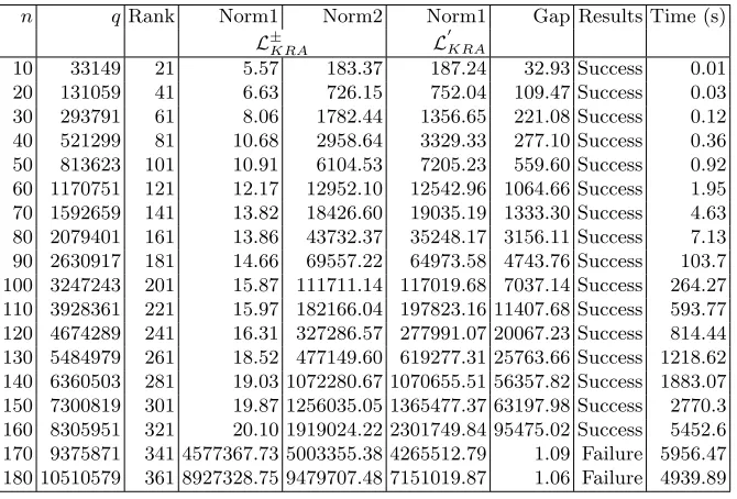
e=(3 0 2 1 0 3 1 2 2 0 2 1). (35) This paper shows computational experiments intended to find the closest vector by the embedding technique.
The embedding technique finds the closest vector from the lattice found by adding the target vector to the original lattice, such as
Ld= ( B 0 dµ ) ,
wheredis a target vector andµis a small integer, such as 1 or 2. When we reduce the latticeLd by applying the LLL or BKZ method, we can find the vectoreas a row vector whose last element equalsµor−µin the reduced lattice.
For the example (27), the embedded lattice is
818 1072 301 264 0 0 371 916 0 0 0 0 0
1072 818 264 301 0 0 916 371 0 0 0 0 0
0 0 818 1072 301 264 0 0 371 916 0 0 0
0 0 1072 818 264 301 0 0 916 371 0 0 0
0 0 0 0 0 0 818 1072 301 264 371 916 0
0 0 0 0 0 0 1072 818 264 301 916 371 0
1459 0 0 0 0 0 0 0 0 0 0 0 0
0 1459 0 0 0 0 0 0 0 0 0 0 0
0 0 1459 0 0 0 0 0 0 0 0 0 0
0 0 0 1459 0 0 0 0 0 0 0 0 0
0 0 0 0 1459 0 0 0 0 0 0 0 0
0 0 0 0 0 1459 0 0 0 0 0 0 0
0 0 0 0 0 0 1459 0 0 0 0 0 0
0 0 0 0 0 0 0 1459 0 0 0 0 0
0 0 0 0 0 0 0 0 1459 0 0 0 0
0 0 0 0 0 0 0 0 0 1459 0 0 0
0 0 0 0 0 0 0 0 0 0 1459 0 0
0 0 0 0 0 0 0 0 0 0 0 1459 0
1223 315 1402 1442 1348 403 425 48 123 179 968 426 2
,
since the vectordis(1223 315 1402 1442 1348 403 425 48 123 179 968 426). Ap-plying LLL to the lattice, we can detect a shortest vector
(