Article
1
Implementation of Smart Tomographic Sensors in
2
Cyber Physical System for Process Analysis in
3
Industry 4.0
4
Tomasz Rymarczyk1,2,*, Grzegorz Kłosowski3, Edward Kozłowski3, Paweł Tchórzewski2
5
1 University of Economics and Innovation in Lublin, Poland; [email protected]
6
2 Research & Development Centre Netrix S.A., Lublin, Poland
7
3 Faculty of Management, Lublin University of Technology, Lublin, Poland; [email protected],
8
9
* Correspondence: [email protected]
10
11
Abstract: The article presents a cyber-physical system for acquiring, processing and reconstructing
12
images from measurement data. The technology was based on process tomography, intelligent
13
measurement sensors, machine learning, Big Data, Cloud Computing, Internet of Things as a
14
solution for Industry 4.0. Industrial tomography enables observation of physical and chemical
15
phenomena without the need of internal penetration and allows real-time monitoring of production
16
processes. The application includes specialized intelligent devices for tomographic measurements
17
and dedicated algorithms for solving the inverse problem. The work focuses mainly on electrical
18
tomography and image reconstruction using deterministic methods and machine learning, the
19
reconstruction results were compared, different measurement models were used. The researches
20
were carried out for synthetic data and laboratory measurements. The main advantage of the
21
proposed system is the possibility of spatial data analysis and their high processing speed. The
22
presented research results show that the process tomography gives the possibility to analyse the
23
processes taking place inside the facility without disturbing the production, analysis and detection
24
of obstacles, defects and various anomalies. Knowing the characteristics of a given solution, the
25
application allows you to choose the appropriate method to reconstruct the image.
26
Keywords: inverse problem; industrial tomography; machine learning, sensors, cyber-physical
27
system, Industry 4.0
28
29
1. Introduction
30
The article presents the results of research on the use of tomographic sensors for the analysis of
31
industrial processes with the use of dedicated measuring devices, image reconstruction algorithms
32
and the cyber-physical system (CPS). Advanced automation and control of production processes play
33
a key role in enterprises. Technological equipment and production lines can be considered the heart
34
of industrial production, while information technologies and control systems are its brain. They
35
ensure high flexibility, fast adaptation of production processes to changing market requirements as
36
well as safety and efficiency with optimal costs of resources and energy. The development and
37
application of advanced mechanisms for process control ensures greater production flexibility.
38
Cyber-Physical Systems is a concept of systems with strictly integrated computational, physical
39
and communication processes. In contrast to advanced systems, CPS create a unified structure for
40
modelling and implementing complex systems as a whole. The presented concept of Cyber Intelligent
41
Enterprise consists directly in the application of the CPS vision in the field of enterprise systems, the
42
Internet of Things (IoT) and the semantic network. The tight integration of physical devices and
43
business processes gives new possibilities and increases the efficiency of the enterprise [1]. Systems
44
of cooperating computing units that are in intense connection with the surrounding physical world
45
and its current processes provide and use simultaneously data access and data access services
46
available on the Internet. They can be part of the fourth industrial revolution, often labelled as
47
Industry 4.0. Cyber-physical production systems (CPPS) are based on the latest developments in the
48
fields of information technology, electronics, information and communication technologies. Such a
49
solution consists of autonomous and cooperating elements and subsystems that connect with each
50
other at all stages of production, from processes through machinery, to production networks and
51
quality control. Autonomy, cooperation, optimization, integration of analytical approaches and
52
simulations is related to the operation of sensor networks, large amounts of data and the search,
53
analysis and interpretation of information with particular emphasis on security aspects [2]. The
54
hybrid NC control system for an automatic line based on CPS technology uses a variety of techniques,
55
such as sensors, intelligent computing and heterogeneous network integration [3]. Integration and
56
intelligence are a development trend of production systems. Using the sensor network, it combines
57
NC production line components, CNC production lines based on real-time information technology
58
updates, intelligent control.
59
60
61
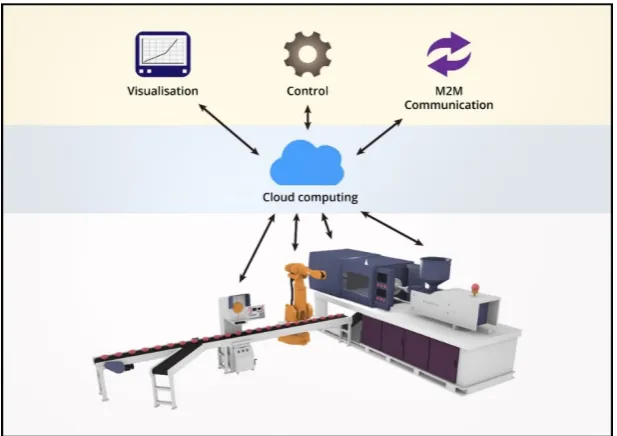
Figure 1. Industrial automation system based on a computing cloud
62
The implementation of a system combining real industrial environments with a virtual copy of
63
components is presented in [4]. The system is based on virtual digital objects with a certain degree of
64
complexity and autonomous control. IoT extends this concept with components of machine
65
communication technology (M2M) and the ability to communicate and interact with physical objects
66
represented by CPS. The system enables communication in the network and performing small tasks
67
in a decentralized way autonomously, which contributes to the personalization of products and
68
adapting the product's functions to local needs and their individual production process (Fig. 1). New
69
technologies offer great opportunities to promote industrial modernization. They allow the
70
introduction of the fourth industrial revolution. In the context of Industry 4.0, all kinds of smart
71
devices supported by wired or wireless networks are commonly used (Fig. 2). Advances in the field
72
of industrial Internet of Things (IIoT) and related fields such as industrial wireless networks (IWN),
73
large data sets and cloud computing help create a new concept for industrial environments. Here one
74
can pay attention to the architecture of the prototype platform deployment, the functions and features
75
of each component layer, and the exchange of information between all types of devices [5]. Intelligent
76
equipment and software are needed to build a smart factory. These include intelligent machine
77
controllers, broadband devices, analytical systems for large data sets and integrated information
78
applications. With the advent of new technologies (IoT, Cloud Computing, Big Data, Artificial
79
Intelligence), intelligent machines and products can communicate with each other and negotiate for
reconfiguration in order to flexibly produce many types of products. Data can be collected from smart
81
devices and transferred to the cloud. This gives feedback and coordination based on the analysis of
82
large data to optimize system performance. Self-organized reconfiguration and communication
83
based on a large amount of data determine the framework and operating mechanism of an intelligent
84
factory in Industry 4.0 [6]. Intelligent production applications based on agents are an appropriate
85
solution to the problem of production planning and scheduling, as production companies can include
86
a variety of different elements, such as production process planning, monitoring and control. The
87
agent-based implementation enables defining workflows and tracking production logic. In
88
automation in production systems, multi-agent technologies can be used for parallel control, using
89
cloud computing and service-oriented architecture (SOA) to share production resources [7].
90
91
92
Figure 2. The idea of the concept of Industry 4.0
93
Tomographic imaging of objects creates a unique opportunity to discover the complexity of the
94
structure without the need to invade the object [8]. There is a growing need for information on how
95
internal flows behave in the process equipment. It should be performed non-invasively by
96
tomographic instrumentation. Conventional measuring instruments may either be unsuitable for
97
difficult internal process conditions or their presence may interfere with the operation of the process.
98
Process tomography is used to manipulate data from remote sensors to obtain precise quantitative
99
information from inaccessible locations. It allows to improve the processes and their design, enabling
100
real-time imaging of the boundaries between different components using non-invasive sensors.
101
Information on substance properties, flow, vector velocity and concentration of ingredients in process
102
vessels and pipelines can be determined based on the images obtained by installing sensors around
103
the object to be imaged. Image data can be analysed online or collected for later use to run a process
104
control strategy or to develop models describing particular processes. Online monitoring and
105
diagnostics on the tomographic data streams can be incorporated into automated decision systems
106
for industrial applications. Computer intelligence methods are capable of solving very complex tasks.
107
Current tomographic systems provide limited support for computer intelligence methods, given the
108
limited space and time of their embedded computational elements. The concept of distributed cloud
109
computing architecture for online processing of tomographic data streams is presented in [9]. The
110
monitored object is a tomographically instrumented part of the production plant, in which the
111
tomographic device collects data by means of exciting electric potentials on its surface in a
non-112
invasive way. The device sends raw data to the cloud computing system, where the inverse problem
113
(image reconstruction) is solved. The final effect is the use of a machine learning algorithm to classify
114
the status of the monitored object and make a specific decision by closing the control loop. Figure 1
115
shows the general scheme of the system operating in a closed loop.
118
Figure 3. A general scheme of a system operating in a closed loop
119
Industrial tomography is a harmless, non-invasive imaging technique used in various industrial
120
technologies to study physical and chemical processes without the need to penetrate their interior. It
121
performs continuous data measurement, it allows better understanding and monitoring of industrial
122
processes, enabling a quick response. This makes it easier to control processes in real time and
123
incorrect system operations. The main advantage of tomographic examinations is their non-invasive
124
nature, which does not cause changes that could interfere with the measurement results. Industrial
125
tomography can be transformed into a powerful sensor solution for control. Distributed
126
infrastructure requires various tasks related to the detection and start-up of processes, and is usually
127
characterized by an internal spatial organization. The wireless sensor network (WSN) technology
128
offers great opportunities in the aspect of cooperation of many devices in a wide range.
129
The presented solution enables the control of processes based on tomographic sensors, analysis
130
of large data sets, multidimensional control of industrial processes, control using advanced
human-131
machine interfaces and monitoring of knowledge-based processes. Sensor technologies are mainly
132
based on electrical tomography (ET) [10-16], which includes capacitance tomography (ECT) [17-25]
133
and resistance tomography (ERT) [26-28]. It allows reconstruction of the image by the distribution of
134
conductivity or permittivity of the object from electrical measurements at the edge of the object.
135
Another method is ultrasound tomography (UT) [29], which is a technique that uses information
136
contained in the ultrasound signal after it passes through the examined object. However, by using a
137
wire mesh sensor (WMS) a distribution of material properties in the gas and liquid flow is obtained
138
in a direct manner. The project is implemented as part of research work at Research and Development
139
Laboratory in Netrix S.A.
140
The article consists of 5 chapters. The architecture of the designed system with the industrial
141
processes and the application platform is presented in Chapter 2. The methods and algorithms used
142
to solve the inverse problem in image reconstruction, numerical models, tomographic devices and
143
laboratory measurement systems are also described here. The results of research work in the form of
144
reconstruction of images for synthetic and measurement data are shown in Chapter 3. In Chapter 4,
145
the results obtained are discussed. Chapter 5 summarizes the research carried out.
146
2. Materials and Methods
147
This chapter presents the system model, tomographic methods, process tomography, measuring
148
devices, laboratory systems, mathematical algorithms and measurement models used in image
149
reconstruction based on synthetic data and real measurements. Laboratory equipment, tomography
150
devices constructed at Research & Development Centre Netrix SA, the Eidors toolbox [30], Microsoft
151
tools, Matlab, Python and R language were used for the research.
2.1. System architecture
153
Advanced control of production processes facilitates modelling of complex relations between
154
process parameters, which guarantees stable, automated and flexible work. The main problem
155
occurring in the research of technologically closed facilities is the lack of information allowing the
156
analysis of the properties and quality of the substance being a component of the technological
157
process. The presented technology allows for monitoring and acquisition of measurements at any
158
time, which is useful for controlling the quality of production processes. Supervision and control take
159
place within the scope of data obtained and processed as well as parameters of executive devices. It
160
will allow to optimize the system in such a way that the processes themselves are always
161
reproducible, leading to further increase of bandwidth, efficiency and quality of products.
162
The solution architecture consists of a cyber-physical system model, measurement sensors and
163
methods for the analysis and classification of algorithms and image reconstruction. The system
164
design was based on containers in the cloud computing model. The use of containers allows the use
165
of public clouds. The use of a distributed system using microservices and containers allows the
166
flexibility of a system in which modules perform clearly defined tasks. The modules are independent
167
of each other, they can be easily replaced with newer versions, and the failure of one of the modules
168
does not cause the whole system to fail. Such architecture will increase the reliability level of the new
169
IT system. It will enable forecasting changes based on the analysis of historical data from the system
170
as well as data obtained from devices in real time. An open platform model for a smart enterprise
171
system (Fig. 4) contains measuring devices for acquiring sensor data, pre-processing and
172
transmission to a system server network (Fig. 5). Another element of the solution is a portal which,
173
together with data exchange interfaces (communication platform), enables management of data
174
stored on the server and will contain documents and processes in the enterprise. Interfaces
175
exchanging data with internal and external systems will participate in the process (Fig. 6). The
176
algorithms of manual and automatic control relate to issues related to data processing, obtained from
177
various sensors located in key nodes of the installation. The main feature of the use of wireless
178
methods is the acquisition of the most important information about the process and installation status
179
in real time by persons who are of strategic importance in the process of management and technical
180
supervision. The transmitted data are analysed by an expert system and are used to optimize
181
production processes (Fig. 7).
182
183
184
Figure 4. An open platform model for a smart enterprise system
186
Figure 5. The communication model between the system elements
187
188
Figure 6. An intelligent system for the production and monitoring of processes
189
190
191
Figure 7. Analysis model of large data sets for machine learning
The central point of the system is a software integration platform that provides instruments for
193
communication and management of smart devices. The platform consists of a communication layer,
194
control software and multi-platform libraries and clients (Fig. 8).
195
196
197
Figure 8. Block diagram of the integration platform of the system used to manage devices
198
From a technical point of view, the platform is scalable, based on microservices implemented on
199
a local hardware platform with the main purpose to work on cloud platforms. The use of the
200
integration platform provides support for the entire process related to device management and data
201
processing. The process consists of stages. from data transfer, validation and collection to processing
202
using algorithms. The integration platform can communicate with devices via the REST
203
(Representational State Transfer) interfaces, the WebSocket (computer communications protocol), or
204
the MQTT (Message Queuing Telemetry Transport) protocol. Almost all devices that support one of
205
these protocols can be connected to the platform.
206
207
208
Figure 9. The structure model of the system for acquisition, processing, data collection and analysis in cloud
209
computing
210
The structure model of the system for acquisition, processing, data collection and analysis in
211
cloud computing was presented in Fig. 9. The data was collected from the devices. The MQTT
212
protocol has been used to transfer data from the source to the analytical system. The data flow was
213
repeated in two flows: the first was transmitted to the database system and the second was sent to
214
the analytical system for further analysis. The purpose of this operation is to process data in real time
215
and to store historical data for additional offline analysis.
2.2. Electrical tomography
218
Electrical tomography is an imaging technique that uses different electrical properties of
219
different types of materials, including biological tissues. In this method, the power or voltage source
220
is connected to the object, followed by the emergence of current flows or the distribution of voltage
221
at the edge of the object. The collected information is processed by an algorithm that reconstructs the
222
image. This tomography is characterized by a relatively low image resolution. Difficulties in
223
obtaining high resolution result mainly from a limited number of measurements, nonlinear current
224
flow through a given medium and too low sensitivity of measured voltages depending on changes
225
in conductivity inside the area. Electrical tomography has historically been divided into electrical
226
capacitive tomography, for systems dominated by dielectrics and electrical resistance tomography.
227
The basic theory can be obtained from Maxwell's equations.
228
A complex 'admittivity' can define as follows:
229
𝛾 = 𝜎 + i𝜔𝜀 (1)
where ε is the permittivity, σ is the electrical conductivity, ω is the angular frequency.
230
In the case of the electric field strength (Ε), the current density (J) in the test area will be related to
231
Ohm's law:
232
𝐽 = 𝛾𝐸 (2)
The gradient of the potential distribution (u) has the form:
233
𝐸 = −∇𝑢 (3)
Due to the fact that there are no sources from the Ampère law in the studied region, we have:
234
∇ ∙ 𝐽 = 0 (4)
Potential distribution in a heterogeneous, isotropic area:
235
∇ ∙ (𝛾∇𝑢) = 0, (5)
where 𝑢 is the potential.
236
Where the capacitance or resistance dominates, the equation factor should be simplified to the form:
237
∇ ∙ (𝜎∇𝑢) = 0 𝑓𝑜𝑟 𝜔𝜀
𝜎 ≪ 1 (ERT) (6)
∇ ∙ (𝜀∇𝑢) = 0 𝑓𝑜𝑟 𝜔ε
𝜎 ≫ 1 (ECT) (7)
By solving the inverse problem, we obtain the distribution of material coefficients in the studied area.
238
Electrical resistance tomography in a process tomography can be interchangeably called electrical
239
impedance tomography (EIT). In the further part of the work, we will mainly use the name EIT
[31-240
35].
241
The opposite method and neighbouring method in EIT for collecting data from potential
242
measurements at the edge of an object for 16 electrodes was shown in Fig. 10.
243
244
(a) (b)
245
Figure 10. Measurement model in electrical impedance tomography: (a) opposite, (b) neighbouring method
In electrical capacitive tomography, the source of information is the electrical capacity between
247
the electrodes located on the edge of the object being tested (see Fig. 11). A very important feature of
248
the measurement in the case of capacitive tomography is the lack of the need for physical interaction
249
of the sensor with the medium being tested, thanks to which this method is non-invasive; that is, it
250
does not disturb the ongoing industrial process. Another advantage of this measuring technique is
251
the fast collection of measurement data. For measurements in capacitive process tomography,
252
specially dedicated systems are used. Due to difficult measurement conditions, it is impossible to use
253
ordinary capacitance measurements. Industrial processes run at high speed, so the measurement
254
must be fast. In addition, the measured capacities are of the order of femtofarad, which requires
255
special measuring techniques.
256
The inverse solution of the problem is achieved:
257
𝜀 = 𝑆 ∗ 𝐶 (8)
where:
258
ε – permittivity matrix
259
C – capacity matrix
260
S – sensitivity matrix
261
Inverse problem can be solved with, for example using the Landweber algorithm:
262
𝜀 = 𝜀 + 𝛼 ∗ 𝑆 ∗ (𝑆 ∗ 𝜀 − 𝐶 ) (9)
where:
263
𝐶 - measured capacity matrix
264
𝜀 – permittivity matrix, current iteration
265
𝜀 – permittivity matrix, previous iteration
266
𝛼 – coefficient
267
268
Figure 11. Measurement model in electrical capacitance tomography
269
2.3. Ultrasund tomography
270
Measurement methods using the information contained in the ultrasonic signal after passing
271
through the tested medium are called ultrasound transmission methods. The main advantage of
272
tomographic examinations is non-invasive measurement in the studied environment, which does not
273
cause changes in physical and chemical parameters that could interfere with the measurement
274
results. The measurement of parameters such as signal transition time, damping coefficient and its
275
derivative by frequency enable, after appropriate reconstructive transformations, the imaging of the
276
internal structure of the tested medium as well as such flow parameters as, for example: its
277
instantaneous velocity, average speed or velocity profile. Differences in the local values of specific
278
acoustic parameters are the basis of this imaging. The image obtained by appropriate reconstruction
279
methods presents, because the distribution of local values of selected acoustic parameters obtained
280
from measuring data by scanning technique from as many directions as possible after the ultrasonic
281
pulses have passed through the tested environment. Ultrasonic transmission tomography for
detecting the two-component high-acoustic impedance mixture is used in chemical columns and
283
industrial pipelines, where solid or gaseous particles inside liquid masses are repeatedly found [36].
284
The tomographic measurement data ensure control of various quality parameters of the material
285
composition. A 2D transmission mode approach was used to reconstruct the acoustic velocity profile.
286
According to the difference in the depth of penetration for given particle concentrations, the signal
287
transit time has been calculated to detect a different material composition in the liquid mass.
288
289
290
Figure 12. Sensor geometry for the ultrasonic tomography measurement system
291
The problem of image reconstruction in the case of ultrasounds leads to the equation in the form of a
292
matrix:
293
𝑊 𝑓 = 𝑠, (10)
where: 𝑠 – right hand side vector (one column matrix), 𝑊 is the matrix of dimensions m x n and
294
m > n, 𝑓 – the solution vector.
295
In order to solve the equation (10) is to find a vector 𝑓, which minimize Euclidean norm of residual
296
vector 𝑟 for the known matrix 𝑊 and vector s, it means:
297
‖𝑟‖ = 𝑚𝑖𝑛‖𝑠 − 𝑊𝑓‖ , ‖𝑓∗‖ = 𝑚𝑖𝑛‖𝑓‖ (11)
where the last minimum is assumed for all vectors 𝑓 that meet the previous relationship.
298
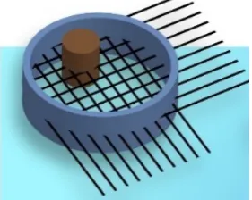
2.4. Wire mesh sensors
299
Wire Mesh Sensor is an invasive instrumentation measuring instantaneous phase distributions
300
in two-phase flows (Fig. 13). WMS consists of two surfaces of wire electrodes; transmitters and
301
receivers. The elements on each WMS plane are stretched parallel to each other and separated by a
302
few millimetres and intersect each other at a 90 ° angle. The measurement of phase distributions is
303
carried out at these intersection points, measuring electrical conductivity to conduct fluids or
304
permeability of non-conductive fluids. On the basis of measurements of conductivity or electrical
305
permeability, the amount of liquid and gas in single-volume components is calculated from the
306
corresponding values [37].
307
308
Figure 13. Model of wire mesh sensor
2.5. Process tomography
310
Process tomography enables the analysis of processes taking place in the facility without
311
interfering with them. It belongs to the opposite problems of the electromagnetic field; its purpose is
312
to determine the properties of the tested object from measurements on its edge [38,39]. It enables
313
better understanding and monitoring of industrial processes and facilitates process control in real
314
time. The main difference in the mass production of chemicals, food and other commodities lies in
315
the fact that common process sensors only provide local measurements. In production systems for
316
the entire process, such local measurements are not representative, therefore spatial solutions are
317
needed. Industrial processes are described in block models of energy and mass exchange elements.
318
Process constituent units with often complex transfer functions derived from empirical process
319
knowledge. The main difference is that a large number of parameter codes loses the spatial prediction
320
capability and thus the current process conditions. In addition, their accuracy decreases, due to their
321
inherent physical complexity in such phenomena as fluid dynamics, crystallization or fermentation
322
process.
323
Data concentration profiles, phases and chemical substances can be investigated with fast data
324
acquisition and image reconstruction. The obtained data can be used to monitor process reactions,
325
improve quality, efficiency and flow rates. They can provide data for on-line process control. Typical
326
industrial applications of process tomography are monitoring of varying concentration profiles in
327
mixing and separation vessels (single-phase and multi-phase). Process tomography can allow you to
328
control and understand processes in real time. It provides up-to-date feedback on processes, their
329
effectiveness and progress in reactions. It can contribute to reducing waste and improving the overall
330
energy efficiency of the company.
331
A change in reaction conditions can lead to a significant increase in production capacity, but it
332
requires a significant change in many aspects of process design and unforeseen difficulties or benefits.
333
The first element is to characterize the individual stages of the process. Process tomography sensors
334
can provide quantitative and qualitative measurements of the dynamics and volume effects of the
335
based processes. The data can be used as basic information about the process. The tomographic
336
sensors can also help determine the efficiency of mixing and other performance characteristics. The
337
tomography can be used to continuously monitor the effectiveness of the process by providing
338
information when the reaction conditions change.
339
The installation of a two-phase flow identification system can be extremely useful in controlling
340
the presence of air bubbles in liquids that are semi-finished products in which the presence of air is
341
unacceptable. The existence of air bubbles in production processes can cause irreversible losses. Also,
342
the presence of air in liquid semi-finished products with higher viscosities in the chemical,
343
pharmaceutical and food industries can be very disadvantageous in some cases. Real-time control to
344
detect the presence of air bubbles.
345
Crystallization is a key reaction in the pharmaceutical sector and other processes. The
346
combination of two ionic species in solution to form a solid part often results in a strong change in
347
electrical properties. The tomographic sensors can study the entire area and provide information on
348
reaction kinetics and concentrations. This can help you pinpoint the reaction endpoints more
349
accurately, as well as provide information on how to ensure the right chemical conditions. The
350
tomographic measurements can also be used in various process ranges to confirm the scale
351
characteristics. Crystallization is a widespread industrial process for the purification of substances
352
and the conversion of dissolved compounds into solid products.
353
Figures 15 and 16 present measurement models for process tomography based on electrical and
354
ultrasonic tomography. Figure 14 presents the idea of system structure with a hybrid tomography
355
scanner with flow measurement, image processing in the cloud computing. The model of analysing
356
the process of crystallization and fermentation is presented in Fig. 17. The UST is more suitable for
357
detecting connections between materials, while ECT better characterizes individual phases. ERT is
358
used to visualize the concentration profile.
361
Figure 15. Measurement model for electrical tomography
362
363
Figure 16. Measurement model for ultrasound tomography
364
365
Figure 14. The idea of system structure with a hybrid tomography scanner with flow measurement, image
366
processing in the cloud computing
367
368
Figure 17. Monitoring, analysis and control processes in the test tank by tomographic methods
369
370
2.6 Measurements systems
372
2.6.1. System model
373
The idea of a measuring system is based on tomographic sensors. The appropriate types of
374
electrodes are placed on the measuring object (Fig. 18). Data acquisition module collects data and
375
through appropriate communication protocols send them to cloud computing, where they are used
376
in tomographic processes.
377
378
Figure 18. The idea of a measurement and analytical system
379
2.6.2. Hybrid tomography scanner
380
The construction of a hybrid tomography scanner was based on an electrical tomography and
381
measures the tested object based on measurements of potential distribution or capacitance. The
382
system collects the measured data from the electrodes. The device provides a non-invasive method
383
of testing the spatial distribution of material coefficients. Presented device for electrical tomography
384
includes two measuring methods using 32 channels. The measurements are based on electrical
385
capacitance tomography and electrical impedance tomography. The device is presented in Figure 19
386
in the form: measuring block, control and communication system, view from the inside and
392
(c) (d)
393
Figure 19. Hybrid tomography scanner: (a) measuring block, (b) control and communication system, (c)
394
view from the inside, (d) measuring panel
395
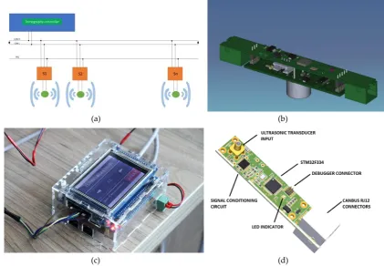
2.6.3. Ultrasound tomography system
396
The ultrasonic tomograph consists of active measuring probes controlled by an external module
397
via a CAN bus. Active measuring probes are divided into digital and analog parts. The digital part is
398
responsible for sending ready measurement results to the tomography controller via the bus. The
399
analog part has been adapted to work with a piezoelectric transducer operating at 48 kHz. The active
400
probe can work both as a receiver of an ultrasonic signal and as a transmitter. The main CT controller
401
is responsible for managing the sequence of measurements, setting up active probes in the transmit /
402
receive mode, and recording results taken from other probes. The probes are designed so that they
403
can be placed very close to each other. Power lines, communication buses and interrupt lines
404
necessary for correct timekeeping from the moment of sending to receiving the signal on other probes
405
were carried out using RJ-12 cables. Figure 20 shows ultrasound tomography device: block diagram,
406
model of measuring probe, start-up control module and active measuring probe.
407
408
409
(a) (b)
410
411
(c) (d)
412
Figure 20. Ultrasound tomography device: (a) block diagram, (b) model of measuring probe, (c) start-up
413
control module, (d) active measuring probe
2.6.4. Wire mesh sensor system
415
Wire mesh sensors are flow imaging devices and enable testing of multiphase flows with high
416
spatial and temporal resolution. Although they could not be considered to belong to the classic
417
tomographic technique because their operating principle relies on unwanted electrodes to generate
418
images, it was considered an alternative technique of previously described tomographic systems. The
419
sensor is a hybrid device between undesirable local measurement of phase fractions and a
420
tomographic section image. The sensor consists of two sets of wires extending in the
cross-421
section of a tank or pipe with a small axial distance between them. Each plane of parallel wires is
422
located perpendicular to each other to form a grid of electrodes. The associated electronics measure
423
the local conductivity in the gaps of all transitions exceeding a high degree of repetition. Considering
424
the two-phase flow, it consisted of an electrically conductive phase and the other non-conductive
425
phase, for example air and water, the obtained conductivity measurements are indications of the
426
phase present at each intersection point. The sensor is able to determine the instantaneous
427
distribution of free fractions in the cross-section. Regarding the principle of measurement, a
428
multiplexer pattern of excitation is used. The wires of one plane are used as transmitters, and the
429
wires of the other plane as receivers. Figure 21 is a block diagram of the electronics of the conductivity
430
grid sensor for an exemplary sensor configuration. Samples from all take-up lines are taken at the
431
same time. This procedure is repeated for all transducer electrodes. The measurements are actually
432
voltages that are proportional to the conductivity of the medium around each intersection of the wire
433
mesh at the time of data extraction. In this way, the grid divides the cross section of the flow channel
434
into several independent subregions, where each intersection constitutes one subregion. Each of the
435
measured signals reflects the flow component in the associated subregion, i.e. each intersection
436
operates as an indicator of the local phase. Thus, the set of data obtained from the sensor directly
437
represents the phase distribution in the cross-section.
438
439
440
Figure 21. System model of wire mesh sensor
441
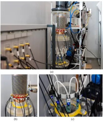
2.7. Laboratory models
442
In the Research and Development Centre of Netrix S.A. measuring stations for liquid flows (Fig.
443
22), the positions for tanks for electrical impedance tomography (Fig. 23) and ultrasound tomography
444
(Fig. 24) were prepared. In this position, the sets of electrodes were placed on the examined objects.
445
Sample image reconstructions made using the ultrasound tomograph are shown in Fig. 25.
448
(a)
449
450
(b) (c)
451
Figure 22. Laboratory model for liquid flows: (a) measuring system, (b) ECT probe, (c) UST probe
452
453
(a) (b)
454
Figure 23. Model of the EIT measurement tank: (a) dimensions, (a) a bucket with electrodes
456
(b) (b)
457
Figure 24. The UST measuring tank: (a) model, (a) real object with the active electrodes
458
459
(c) (b) (c) (d)
460
Figure 25. Examples of reconstruction using UST for 20 measuring points with 48 kHz transducers: (a) 1
461
phantom, (a) image reconstruction for 1 object, (a) 3 phantoms, (a) image reconstruction for 3 objects
462
2.8. Measurement models
463
In order to test the effectiveness of algorithms for the analysis of processes in industrial
464
tomography, three measuring models were selected. Electrical tomography was used for the analysis.
465
The arrangement of phantoms inside the object under test were presented in Fig. 26. The measuring
466
tank is shown in Fig 27.
467
468
469
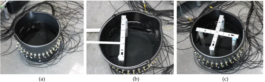
(a) (b) (c)
470
Figure 26. The arrangement of phantoms inside the object under test: (a) 2 phantoms, (a) 3 phantoms, (a) 4
471
phantoms
473
(a) (b) (c)
474
Figure 27. Measuring tank: (a) bucket with electrodes, (a) 2 phantoms, (a) 4 phantoms
475
2.9. Numerical models
476
An important element in the process of testing the effectiveness of algorithms is the preparation
477
of numerical models. They were prepared in two variants: for 16 and 32 electrodes (Fig. 28 and Fig.
478
29).
479
480
481
(a) (b) (c)
482
Figure 28. Numerical models for 16 measuring electrodes: (a) 2 objects, (b) 3 objects, (c) 4 objects
483
484
485
(a) (b) (c)
486
Figure 29. Numerical models for 32 measurement electrodes: (a) 2 objects, (b) 3 objects, (c) 4 objects
487
2.10. Algoruthms and methods
488
There are many methods and algorithms used in optimization problems [40-51]. In this article,
489
the authors chose deterministic algorithms based on the Gauss-Newton and Total Variation methods,
490
often used and quite effective in electrical tomography. The next algorithms were based on machine
491
learning method [52-56]s, in which an innovative approach to tomographic problems was presented.
2.10.1. Image reconstruction
494
Process tomography also belongs to the problems of the inverse electromagnetic field. The
495
inverse problem is the process of optimization, identification, or synthesis in which the parameters
496
describing a given field are determined based on the possession of information specific to this field.
497
Such issues are difficult to analyse. They do not have unambiguous solutions and are ill-conditioned
498
due to too little or too much information. They are sometimes contradictory or linearly dependent.
499
Knowledge of the process can make image reconstruction more resistant to incomplete or damaged
500
data. The numerical analysis of the problem was carried out using the finite element method.
501
2.10.2. Gauss-Newton method
502
The Gauss-Newton Method is a very effective method. It is based on the first derivatives of the
503
vector function components implemented. In special cases, it may give a square convergence [57].
504
Electrical tomography is a nonlinear problem, and it has an inverse ill-posed problem. Gauss-Newton
505
algorithm can use to minimize differences between homogeneous and heterogeneous data [58].
506
Image reconstruction involves determining the global minimum of the objective function, which can
507
be defined as follows:
508
𝐹(𝜎) = 𝐿 𝑈 − 𝑈 (𝜎) + 𝜆 ‖𝐿 (𝜎 − 𝜎∗)‖ , (12)
where:
509
Um - voltages obtained as a result of the measurements,
510
Us(σ) - voltages received by numerical calculations (FEM),
511
σ - conductivity,
512
σ* - conductivity represents known properties,
513
λ - regularization parameter - positive real number,
514
L1 - some square matrix,
515
L2 - regularization matrix.
516
Using appropriate approximations, it can be shown that the conductivity proper in the iteration
517
denoted by k + 1 is given by the following formula:
518
𝜎 = 𝜎 + 𝛼 (𝐽 𝑊 𝐽 + 𝜆 𝑊 ) 𝐽 𝑊 𝑈 − 𝑈 (𝜎 ) − 𝜆 𝑊 (𝜎 − 𝜎∗) , (13)
where: W1 - weighting matrix - it is usually a unit matrix, Jk - Jacobian matrix calculated in k-th step,
519
αk - step length.
520
2.10.3. Total Variation
521
In machine learning and inverse problems, regularization provides additional information to
522
solve the problem. Representative information is considered by introducing a penalty function based
523
on constraints for a given solution or boundaries in the vector space standard. Certain cases of
524
statistical regularization include methods such as dorsal regression, lasso and L2 norm. The concept
525
of regularization is based on the application of standards. Total Variation (TV) regularization is a
526
deterministic technique that protects discontinuities [59]. The Total Variation algorithm is used to
527
maintain the discontinuity value on the resulting reconstruction, so that the obtained images have
528
sharp edges at the discontinuity.
529
The objective function can be defined as follows:
530
𝐹(σ) = ‖ 𝑈 (σ) − 𝑈 ‖ + 𝜆 ∑ | 𝑅 σ |, (14)
where:
531
λ - regularization parameter,
532
Ri - a row vector that represents a discrete approximation of the gradient operator,
533
N - number of finite element mesh edges.
2.10.4. Lars
536
Machine learning is related to the ability of the software to generalize based on previous
537
experience. The important thing is that these generalizations are designed to answer questions about
538
both previously collected data and new information. Using statistical methods with different
539
regression models were presented in [60]. This approach enables quick diagnosis combining low cost
540
and high efficiency. The selection of variables and the detection of data anomalies are not separate
541
problems. To use the variables and outliers at the same time, the low angle regression (LARS)
542
algorithm is used. While it is prudent to be cautious about the generalization of a small set of
543
simulation results, it seems that LARS combined with dummy variables or row samples can provide
544
computationally efficient, robust selection procedures [61]. The proposed LARS algorithm calculates
545
all possible Lasso estimates for a given problem using an order of magnitude of less computing time.
546
Another variation of LARS implements the linear regression of Forward Stagewise, this combination
547
explains similar numerical results previously observed for Lasso and Stagewise and helps to
548
understand the properties of both methods. A simple approximation of LARS degrees of freedom is
549
available, from which the estimated prediction error value [62] is taken.
550
If the regression data has only additional outliers, then we can start with a simple regression model:
551
𝑌 = 𝑋𝛽 + 𝜀, (15)
where 𝑌 ∈ 𝑅 , 𝑋 ∈ 𝑅 ×( ) denote the observation matrices of response and input variables
552
respectively, 𝛽 ∈ 𝑅 denotes the vector of unknown parameters. The object 𝜀 ∈ 𝑅 presents a
553
sequence of disturbances. Least Angle Regression algorithm includes to linear model only causal
554
variables should be included. The linear model is built by employing the forward stepwise
555
regression, where at each step the best variable is inserted to model.
556
Algorithm of Least Angle Regression is following:
557
• the predictors should be standardized,
558
• calculate the residuals,
559
• move coefficient β towards its least-squares coefficient.
560
Repeat until all predictors have been entered.
561
2.10.5. Elastic net
562
Elastic net is a regularized regression method that linearly combines the L1 and L2 penalties of
563
the Lasso and ridge methods [63-66]. Lasso is a regularization technique. This method can be used to
564
reduce the number of predictors in a regression model or it selects among redundant predictors.
565
The equation is used to determine the linear regression:
566
min
( , )∈ ∑ (𝑦 − 𝛽 − 𝑥 𝛽 ) + 𝜆𝑃 (𝛽 ), (16)
where 𝑥 = (𝑥 , … , 𝑥 ), 𝛽 = (𝛽 , … , 𝛽 ) for 1 ≤ 𝑖 ≤ 𝑛 and 𝑃 is an elastic net penalty
567
𝑃 is defined as:
568
𝑃 (𝛽 ) = (1 − 𝛼) ‖𝛽 ‖ + 𝛼‖𝛽 ‖ = ∑ 𝛽 + 𝛼 𝛽 , (17)
We see that the punishment is a linear combination of norms 𝐿 and 𝐿 of unknown parameters𝛽.
569
The introduction of the parameter-dependent penalty function to the objective function reduces the
570
estimators of unknown parameters.
571
2.10.6. Neural Network
572
This chapter presents the neuronal model enabling efficient reconstruction of tomographic
573
images. Effective use of artificial neural networks in tomography is possible, but the effectiveness of
574
this tool depends on many conditions. First of all, ANN (artificial neural networks) are able to
575
effectively visualize objects, many of which are already known. A characteristic feature that
576
distinguishes the discussed model is the separate training of neural networks in the amount equal to
the resolution of the output image grid. A suitable model of a neural tomographic system is shown
578
in Fig. 30.
579
580
Figure 30. A mathematical neural model for converting electrical signals into images
581
3. Results
582
This chapter presents the results of image reconstruction based on built numerical models and
583
laboratory measurements. Data analysis is an important part of the diagnosis of the process based on
584
tomography. Knowledge of the process can make the image reconstruction better. Inside the area, a
585
mesh of finite elements is generated. As a result of the calculations it obtains a reconstructed image.
586
The inverse problem was solved using deterministic methods and machine learning.
587
3.1. Image reconfiguration for syntetic data
588
3.1.1. Gauss-Newton method
589
The Gauss-Newton method in two variants was used to reconstruct the image in the electrical
590
tomography for the 16 and 32 electrode systems. The first model includes Laplace regularization
591
(Figures 31 and 32), while the second variant has Tikhonov regularization (Figures 33 and 34).
592
Reconstructed objects show models with 2, 3 and 4 inclusions.
593
594
595
(a) (b) (c)
596
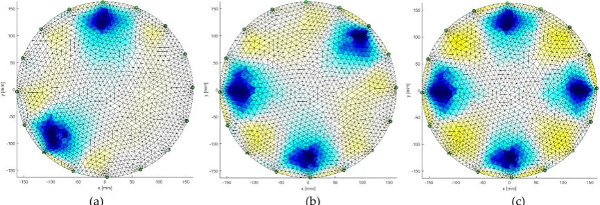
Figure 31. Image reconstruction for 16 measurement electrodes by Gauss-Newton method with Laplace
597
regularization: (a) 2 objects, (b) 3 objects, (c) 4 objects
599
(a) (b) (c)
600
Figure 32. Image reconstruction for 32 measurement electrodes by Gauss-Newton method with Laplace
601
regularization: (a) 2 objects, (b) 3 objects, (c) 4 objects
602
603
(a) (b) (c)
604
Figure 33. Image reconstruction for 16 measurement electrodes by Gauss-Newton method with Tikhonov
605
regularization: (a) 2 objects, (b) 3 objects, (c) 4 objects
606
607
(a) (b) (c)
608
Figure 34. Image reconstruction for 32 measurement electrodes by Gauss-Newton method with Tikhonov
609
regularization: (a) 2 objects, (b) 3 objects, (c) 4 objects
610
3.1.2. Total Variaton method
611
Image reconstruction using the Total Variation method for a system with 16 measuring
612
electrodes is shown in Fig. 35. We obtain a better reconstruction quality in Fig. 36 with 32 measuring
613
electrodes.
616
(a) (b) (c)
617
Figure 35. Image reconstruction for 16 measurement electrodes by Total Variation method: (a) 2 objects, (b)
618
3 objects, (c) 4 objects
619
620
(a) (b) (c)
621
Figure 36. Image reconstruction for 32 measurement electrodes by Total Variation method: (a) 2 objects, (b)
622
3 objects, (c) 4 objects
623
3.1.3. Neural Networks
624
Image reconstruction in the case of neural networks depends largely on the training set.
625
Therefore, reconstructions for an object with 16 electrodes (Fig. 37) gave better results than for an
626
object with 32 electrodes (Fig. 38).
627
628
629
(a) (b) (c)
630
Figure 37. Image reconstruction for 16 measurement electrodes by Neural Networks: (a) 2 objects, (b) 3
631
objects, (c) 4 objects
633
(a) (b) (c)
634
Figure 38. Image reconstruction for 32 measurement electrodes by Neural Networks: (a) 2 objects, (b) 3
635
objects, (c) 4 objects
636
3.1.4. Lars
637
Another algorithm was based on the Lars method. A teaching set of 5000 elements was used
638
here only. In this case, the obtained results for a system with 16 electrodes (Fig. 39) are slightly worse
639
than for a system with 32 electrodes (Fig. 40). The key element in this method is the separation of a
640
group of independent measurements.
641
642
(a) (b) (c)
643
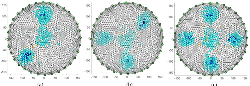
Figure 39. Image reconstruction for 16 measurement electrodes by Lars: (a) 2 objects, (b) 3 objects, (c) 4
644
objects
645
646
(a) (b) (c)
647
Figure 40. Image reconstruction for 32 measurement electrodes by Lars: (a) 2 objects, (b) 3 objects, (c) 4
648
objects
649
650
3.1.5. Elastic net
652
The final algorithm is Elastic net, it is more universal due to its character and gives quite precise
653
results. The same teaching set was used as for the previous method. Reconstructions for systems with
654
16 and 32 electrodes are shown in Fig. 41 and Fig. 42, respectively.
655
656
657
(a) (b) (c)
658
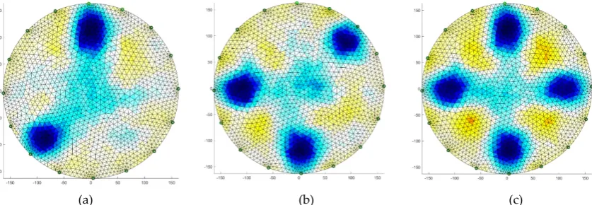
Figure 41. Image reconstruction for 16 measurement electrodes by Elastic net: (a) 2 objects, (b) 3 objects, (c)
659
4 objects
660
661
(a) (b) (c)
662
Figure 42. Image reconstruction for 32 measurement electrodes by Elastic net: (a) 2 objects, (b) 3 objects, (c)
663
4 objects
664
3.1.6. Comparison of image reconstruction
665
The summary of the presented image reconstructions for the indicated methods (Gauss-Newton,
666
Total Variation, Neural Networks, Lars and Elastic net) with 4 unknown objects for the measurement
667
system with 16 electrodes is Figure 43
668
669
670
(a) (b) (c)
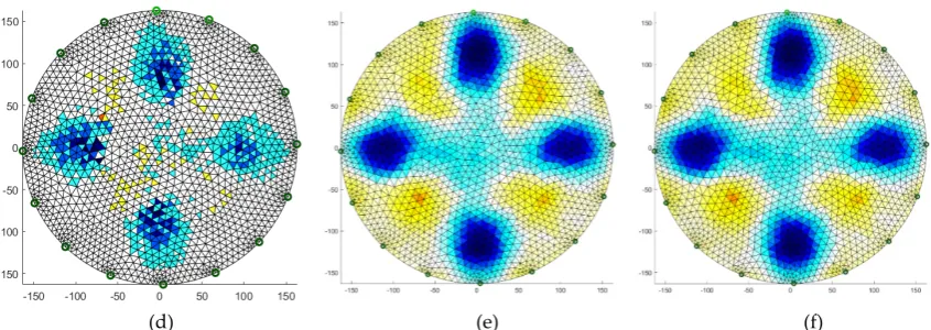
672
(d) (e) (f)
673
Figure 43. Summary of image reconstruction for different methods with 4 unknown objects- measuring
674
system with 16 electrodes: (a) Gauss-Newton with Laplace regularization, (b) Gauss-Newton with
675
Tikhonov regularization, (c) Total Variation, (d) Neural Networks, (e) Lars, (f) Elastic net
676
3.2. Image reconstruction for small objects
677
The analysis of processes in which there are a large number of smaller objects is of great
678
importance in the tomography. For this purpose, individual methods have been analysed on several
679
examples. Figure 44 presents the image reconstruction by using the deterministic method in EIT
680
model. Reconstruction using the Lars method in ECT is shown in Figure 45. In contrast, the elastic
681
net method was implemented for the EIT model in Figure 46. Also, for the EIT method reconstruction
682
was performed using multiply Neural Networks (Fig. 47). Figure 48 shows a comparison of
683
reconstructions for EIT and ECT using the elastic net method.
684
685
686
(a) (b)
687
688
(a) (b)
689
Figure 44. Image reconstruction - EIT model: (a) pattern, (b) Gauss-Newton method with Tikhonov
690
regularization, (c) Gauss-Newton method with Laplace regularization, (d) Total Variation
692
693
(a) (b)
694
Figure 45. Image reconstruction – ECT model: (a) pattern, (b) Lars
695
696
697
(a) (b)
698
Figure 46. Image reconstruction – EIT model: (a) pattern, (b)Elastic net
700
701
(a) (b)
702
Figure 47. Image reconstruction – EIT model: (a) pattern, (b) multiply Neural Network
703
704
705
(a) (b) (c)
706
Figure 48. Image reconstruction by Elastic net: (a) pattern, (b) ECT, (c) EIT
707
3.3. Hybrid EIT/ECT
708
In order to improve the quality of reconstructed images, this chapter uses a hybrid combination
709
of measurement data from the EIT and ECT methods. Figure 49 presents the results using the elastic
710
net method, while Figure 50 shows reconstruction using the multiply Neural Network. A larger
711
amount of input data has improved the quality of image reconstruction, especially after the use of
712
multiply Neural Network.
715
716
(a) (b)
717
Figure 49. Image reconstruction – hybrid model: (a) pattern, (b) Elastic net
718
719
720
(a) (b)
721
Figure 50. Image reconstruction – hybrid model: (a) pattern, (b) multiply Neural Network
722
723
3.4. Image reconstruction by laboratory measurements
725
Figures 51-56 present the results of reconstruction of images based on laboratory measurements
726
of the examined objects. The measuring models are described in section 2.8. A system with 16
727
electrodes was used here. Deterministic methods effectively reconstruct the image based on real
728
measurements. The results obtained using neural networks depend to a large extent on the training
729
set, therefore the quality of reconstruction is not ideal. The Lars method is quite sensitive, while
730
Elastic net is quite universal, because by selecting the appropriate regularization parameters you can
731
get enough good reconstructions on the actual data.
732
733
734
(a) (b) (c)
735
Figure 51. Reconstruction of images based on real measurements by Gauss-Newton method with Laplace
736
regularization: (a) 2 objects, (b) 3 objects, (c) 4 objects
737
738
(a) (b) (c)
739
Figure 52. Reconstruction of images based on real measurements by Gauss-Newton method with Tikhonov
740
regularization: (a) 2 objects, (b) 3 objects, (c) 4 objects
741
742
(a) (b) (c)
743
Figure 53. Reconstruction of images based on real measurements by Total Variation: (a) 2 objects, (b) 3
744
objects, (c) 4 objects
746
(a) (b) (c)
747
Figure 54. Reconstruction of images based on real measurements by Neural Network: (a) 2 objects, (b) 3
748
objects, (c) 4 objects
749
750
(a) (b) (c)
751
Figure 55. Reconstruction of images based on real measurements by Lars: (a) 2 objects, (b) 3 objects, (c) 4
752
objects
753
754
(a) (b) (c)
755
Figure 56. Reconstruction of images based on real measurements by Elastic net: (a) 2 objects, (b) 3 objects,
756
(c) 4 objects
757
4. Discussion
758
4.1. Distributed tomography system
759
Research work presents the original concept of a complex system based on smart tomographic
760
sensors, a cyber-physical system for process analysis in Industry 4.0. The results of the research
761
present the use of tomographic sensors for the analysis of industrial processes using dedicated
762
measuring devices and image reconstruction algorithms. The presented system architecture will
763
increase the level of reliability and efficiency of technological processes in the enterprise. It will enable
764
forecasting changes based on real-time data analysis and historical data. The communication