Eleventh Floor, Menzies Building Monash University, Wellington Road CLAYTON Vic 3800 AUSTRALIA
Telephone: from overseas:
(03) 9905 2398, (03) 9905 5112 61 3 9905 2398 or 61 3 9905 5112
Fax:
(03) 9905 2426 61 3 9905 2426
e-mail: [email protected]
Internet home page: http//www.monash.edu.au/policy/
Development of a large-scale single U.S.
region CGE model using IMPLAN data:
A Los Angeles County example with a
productivity shock application
by
J.A.
GIESECKE
Centre of Policy Studies
Monash University
General Paper No. G-187 August 2009
ISSN 1 031 9034 ISBN 0 7326 1594 1
i
Development of a large-scale single U.S. region CGE model using IMPLAN data: A Los Angeles County example with a productivity shock application
J.A. Giesecke*
Centre of Policy Studies, Monash University
Abstract
This paper details the construction of a large-scale computable general equilibrium (CGE) model for a single U.S. region. The model contains detailed treatment of margins and taxes, features not typically given prominence in U.S. regional CGE models. The starting point for the core of the CGE model’s data base is information from IMPLAN, producers of regional I/O data at the U.S. county and state levels. IMPLAN’s I/O tables, however, are in producer prices with aggregated treatment of margins and taxes. The methods for reconfiguring the I/O data into basic price flows with direct allocation of imports and a disaggregated treatment of taxes and margins are described. The method is applied to construction of a Los Angeles County model. An illustrative simulation of a productivity improvement in the Los Angeles County economy is then discussed.
JEL Classification: C68, R13, R15
Key words: regional CGE, IMPLAN.
* Postal address: James Giesecke, Centre of Policy Studies, Monash University, Clayton Melbourne, Australia 3800.
Ph: +61 3 9905 9756 Fax: +61 3 9905 2426
iii
1. INTRODUCTION 1
2. A SUB-NATIONAL IMPLEMENTATION OF THE ORANI MODEL 1
2.1 ORANI-R model overview 1
2.2 Development of a sub-national implementation of ORANI-G 2
2.2.1 Short-run and long-run regional labour supply 2
2.2.2 The price of interstate and foreign imports. 3
2.2.3 Imperfect substitution between commodity varieties. 4
2.2.4 Interstate and foreign export demand. 4
3. CONSTRUCTION OF AN ORANI-R DATABASE FROM IMPLAN DATA 6
3.1. Step 1: A single region producer price IO table from IMPLAN 7 3.2. Step 2: Conversion of the IMPLAN producer price table to a
basic price table 9
3.3. Step 3: Preliminary identification of margin matrices 11
3.4. Step 4: Disaggregation of investment by industry 13
3.5. Step 5: Construction of tax and margin matrices related
to intermediate inputs 15
3.6. Step 6: Construction of tax and margin matrices related
to private consumption 16
3.7. Step 7: Construction of tax and margin matrices related
to destination-specific exports 17
3.8. Step 8: Construction of tax and margin matrices related
to state and federal public consumption 19
4. SHORT- AND LONG-RUN CONSEQUENCES OF PRODUCTIVITY
GROWTH IN THE LOS ANGELES COUNTY ECONOMY 20
4.1 Simulation design 20
4.2 Short-run consequences of a 1 per cent improvement in primary factor
productivity 21 4.3 Long-run consequences of a 1 per cent improvement in primary factor
productivity 22
5. CONCLUSIONS 24
1
1. INTRODUCTION
IMPLAN (Minnesota IMPLAN Group 1997) is a widely-used data resource for undertaking input-output analysis at the U.S. sub-regional level. ORANI-G (Horridge 2003) is a widely-used template for a detailed single-region CGE model. This paper uses IMPLAN data, together with share and parameter values from USAGE1, to construct a single-region CGE model for a small U.S. region. To make ORANI-G (a single country model) suitable for implementation at the small region level, a number of theoretical modifications to the standard ORANI-G framework are necessary. These are described in Section 2. The resulting model is called ORANI-R. Section 3 describes the development of the ORANI-R database from IMPLAN data. The specific implementation is Los Angeles County. Section 4 presents an illustrative simulation with the new model: short-run and long-short-run productivity growth in the Los Angeles County economy.
2. A SUB-NATIONAL IMPLEMENTATION OF THE ORANI MODEL 2.1 ORANI-R model overview
The well-known ORANI-G model is used as the starting point for the development of a single-region sub-national model, ORANI-R. The structure of ORANI-R is identical to that of ORANI-G in all respects other than those outlined in Section 2.2. Full documentation of the theoretical structure of ORANI-G and its antecedent, ORANI, are available in Horridge (2003) and Dixon et al. (1982) respectively.
ORANI-R is a single-region sub-national comparative-static computable general equilibrium model. The model features detailed sectoral disaggregation. For example, the Los Angeles County implementation developed in this paper covers 436 sectors and 19 margin commodities. Familiar neoclassical assumptions govern the behaviour of the model’s economic agents. Decision-making by firms and households is governed by optimising behaviour. Each representative industry is assumed to minimise costs subject to constant returns to scale production technologies and given input prices. Household commodity demands are modelled via a representative utility-maximising household. Units of new industry-specific capital are assumed to be cost minimising combinations of commodities sourced from the local region, the rest of the U.S. and overseas. Imperfect substitutability between local, rest-of-U.S. and foreign varieties of each commodity are modelled via CRESH2 aggregation functions. Inter-regional and foreign export demands for local commodities are modelled via commodity- and destination-specific constant elasticity export demand schedules. The model recognises the consumption of commodities by state and federal government. A variety of direct and indirect taxation instruments are identified. Domestic commodity markets are assumed to clear and to be competitive. Purchasers’ prices differ from basic prices by the value of indirect taxes and
1 USAGE is a detailed, dynamic CGE model of the U.S. It has been developed at the Centre of Policy
Studies, Monash University, in collaboration with the U.S. International Trade Commission. Prominent applications of USAGE by the U.S. International Trade Commission include USITC (2004 and 2007)
2
margin services. The model is solved using the GEMPACK economic modelling software (Harrison and Pearson, 1996).
2.2 Development of a sub-national implementation of ORANI-G
To date, ORANI has only been implemented as a national model. To implement the ORANI model at the sub-national level, new theory must be added to the core model to determine:
(i) short-run and long-run regional labour supply; (ii) the price of interstate imports;
(iii) the price of interstate exports;
(iv) imperfect substitution between commodity varieties.
These developments are discussed below.
2.2.1 Short-run and long-run regional labour supply
A typical labour market closure for a single-country short-run implementation of the ORANI model assumes endogenous national employment with an exogenous real consumer wage. This setting is suitable for short-run modelling of countries with centralised wage setting arrangements and moderate or high unemployment. It is less suitable in situations of decentralised wage setting and low unemployment. As such, the single-region U.S. implementation of ORANI-G proposed in this paper establishes a regional labour market theory and closure that allows simultaneous stickiness in short-run employment and wages. This better-reflects a short-run situation of low unemployment, stickiness in regional migration, and wage flexibility: characteristics of the U.S. labour market3. The following four equations describe the regional labour market:
(1) pprate=αPPRATE×realwage+ fPPRATE
(2) emprate=αEMPRATE×realwage+ fEMPRATE
(3) hours=αHOURS×realwage+ fHOURS
(4) pop=αPOP×(realwage− frealwage)+ fPOP
(5) employ= pop+shwrkage+pprate emprate hours+ +
where:
3 It also facilitates short-run exogenous shocks to regional labour supply, something not possible under an
3
pprate is the percentage change in the regional participation rate;
realwage is the percentage change in the regional real wage;
PPRATE
f is a shifter on equation (1), typically exogenous;
emprate is the percentage change in the regional employment rate (1 – the
unemployment rate);
EMPRATE
f is a shifter on equation (2), typically exogenous;
hours is the percentage change in hours worked per worker;
HOURS
f is a shifter on equation (3), typically exogenous;
pop is the percentage change in the regional population;
frealwage is a vertical (regional wage premium) shifter on equation (4);
POP
f is a shifter on equation (4);
shwrkage is the percentage change in the share of the regional population that is of
working age;
employ is the percentage change in regional employment;
PPRATE
α is the elasticity of the regional participation rate to the real wage;
EMPRATE
α is the elasticity of the regional employment rate to the real wage;
HOURS
α is the elasticity of hours worked per worker to the real wage; and
POP
α is the elasticity of regional population to the real wage.
A short-run closure of equations (1) – (5) has fPPRATE, fEMPRATE, fHOURS, frealwage,
pop, and shwrkage exogenous, with pprate, emprate, hours, fPOP and employ
endogenous. realwage is determined endogenously in ORANI-R, but largely outside the system of equations (1) – (5). Under this labour market closure, regional population is fixed. This largely ties-down regional employment via equation (5). However some scope for short-run regional employment change is nevertheless provided by equations (1) – (3). These allow for short-run movements in participation, the employment rate, and hours worked per worker, in response to movements in the real consumer wage. The long-run labour market closure is identical to the short-run closure in all respects other than provision for regional population to be a positive function of the regional real wage via activation of equation (4). Equation (4) is activated by exogenous determination of
POP
f and endogenous determination of pop.
2.2.2 The price of interstate and foreign imports.
4 (6) (0), ,[ / ] (0),
t t
c s c s r US c s
p =η GDP GDP x (s = rest-of-U.S., foreign)
(t = short-run, long-run)
where:
(0) ,
t c s
p is the percentage change in the basic price of commodity c from foreign
and rest-of-U.S. sources over length of run t.
,
t c s
η is the reciprocal of the elasticity of supply of imported commodity c
from source s over length of run t. For ,
t c foreign
η we use USAGE database values for the elasticity of U.S. foreign import prices to U.S. import demand. For ηc rest of U Sshort run, −− − . . we derive short-run U.S. commodity-specific
supply elasticities from the USAGE database via the formula of Dixon
et al. (1982: 309). For long-run applications we set long run, . .
c rest of U S η −
− − at one
third of its short-run value. /
r US
GRP GDP is the ratio of regional GDP in the region for which the ORANI-R
model is implemented relative to total U.S. GDP. For example, in the Los Angeles County implementation reported in Sections 3 and 4, this value is 0.037.
(0) ,
c s
x is the percentage change in demand for commodity c from source s.
2.2.3 Imperfect substitution between commodity varieties.
The G model identifies two commodity sources: domestic and foreign. ORANI-R identifies three commodity sources: local, interregional and foreign. In OORANI-RANI-ORANI-R, imperfect substitution between competing sources for the same commodity is modelled via CRESH aggregation functions (Hanoch, 1971)4.
2.2.4 Interstate and foreign export demand.
Prices of regional exports, foreign and domestic, are determined via constant elasticity export demand functions, as follows:
(7) (4) (4) (4)
, , ,
c d c d c d
x =η ×p
where
(4) ,
c d
x is the percentage change in the volume of regional exports of c to destination d (d
= rest-of-US (RUS), foreign);
(4) ,
c d
η is the price elasticity of demand for exports of commodity c to destination d; and
(4) ,
c d
p is the percentage change in the purchaser’s price of commodity c in destination d.
4 Use of CRESH to model commodity-sourcing in a multi-regional framework was first made by Madden
5
In evaluating ηc RUS(4), ., we assume that agents in the rest of the U.S. (RUS) face CRESH
substitution possibilities across three commodity sources: the ORANI-R region, the rest of the U.S., and overseas. This is consistent with the modelling of commodity sourcing for agents within the region of ORANI-R implementation (see 2.2.3 above). With demands for the region’s commodities determined via CRESH aggregation functions in the rest of the U.S., demands for the region’s exports in the rest of the U.S. (RUS) are determined by5:
(8) (4), ( ) (,interregional) ( (4), (4), ( ) (4), (4), )
RUS RUS RUS
c RUS c c c RUS c RUS c c RUS c RUS
x =x −σ Φ p −S Φ p
where,
(4) ,
c RUS
x is the percentage change in the region’s exports of good c to the rest of the
U.S. (RUS);
(RUS)
c
x is the percentage change in demand for good c in the rest of the U.S. (RUS), undifferentiated by source;
( ) ,interegional
RUS c
σ is the CRESH substitution elasticity in the rest of the U.S. (RUS) for good c
sourced from the region of focus;
(4) ,
c RUS
Φ is the share of the f.o.b price of inter-regional export c in the purchaser’s price of c in the rest of the U.S (RUS);
(4) ,
c RUS
p is the percentage change in the f.o.b. price of good c exported to the rest of the U.S. (RUS) from the region of focus; and
(RUS)
c
S is the share of good c from the region of focus in total usage of good c in the rest of the U.S. (RUS).
Assuming (RUS)
c
x is independent of activity in the region of focus, equation (8) implies an inter-regional export demand elasticity for good c of:
(9) (4) ( ) (4) ( )
, ,interregional , (1 )
RUS RUS
c RUS c c RUS Sc
η = −σ Φ −
In evaluating (9), the CRESH substitution elasticity on cross-border intra-U.S. sourcing in the rest of the U.S. ( (,interregional)
RUS c
σ ) is set at the same value as that in the region of focus6. The share of the f.o.b price of c in the purchaser’s price (Φ(4)c RUS, ) is set at 0.8. The share of c in the rest of the U.S. that is sourced from the region of focus (Sc(RUS)) is evaluated via comparison of USAGE values for U.S. demand for c and IMPLAN values for inter-regional exports of c by the region of focus.
5 See Dixon et al. (1992: 128) for derivation of the percentage change form of cost-minimising CRESH
input demands.
6
In evaluating ηc foreign(4), ., use is made of commodity-specific export demand elasticities
from the economy-wide model USAGE. At the same time, a floor is placed on the potential elasticity value via an assumption that agents in other countries face CES inter-regional substitution possibilities. Hence, ηc foreign(4), . is set via:
(10) (4) (4) (4) (4)
, [ [ / ], 6.4]
USAGE USA REG c foreign MAX c Vc Vc
η = η × −
where:
(4)USAGE c
η is the foreign export demand elasticity for commodity c in the USAGE model. A typical value for ηc(4)USAGE is -3.
(4)USA c
V is the national value of U.S. exports of c.
(4)REG c
V is the value of foreign exports of c by the region of focus.
A floor of -6.4 is set on foreign export demand elasticities by reference to Anderson et al. (2008). They show that if foreign agents face sourcing substitution possibilities described by the World Bank’s LINKAGE model (van der Mensbrugghe 2005), the minimum export demand elasticity is given by (2) FOB
i Si
φ , where (2)
i
φ is the elasticity of substitution between alternative foreign sources of supply for imported good i, and SiFOB is the share of the f.o.b price in the foreign country purchaser’s price of good i7. A typical LINKAGE value for φi(2) is 8. With
FOB i
S set at 0.8, this establishes the -6.4 floor on commodity-specific foreign export demand elasticities in equation 10.
3. CONSTRUCTION OF AN ORANI-R DATABASE FROM IMPLAN DATA
The ORANI-R model described in Section 2 has the following characteristics: 1. the structure of capital formation is distinguished by industry;
2. there are three sources of commodity supply: local, rest of U.S., and foreign; 3. there are two export destinations: rest of U.S., and foreign;
4. public consumption is distinguished by whether it is undertaken by the regional government or the federal government; and
5. purchasers’ prices differ from basic prices by the value of margins and indirect taxes.
An initial solution to such a model is provided by a balanced input-output table with the following characteristics:
1. a basic price valuation basis;
2. use of services as margins distinguished from direct use of those commodities; 3. investment demand disaggregated by industry;
4. public consumption demand distinguished by government; 5. export demand distinguished by destination; and
7
6. commodity, source and user specific taxes and margins.
Such an input-output table is described by Figure 8. Sections 3.1 – 3.8 describe steps in constructing such a table, using IMPLAN producer price tables and relevant shares from the USAGE database.
3.1. Step 1: A single region producer price IO table from IMPLAN
Figure 1 reports the structure of the disaggregated single-region input-output table that can be constructed from IMPLAN data. The table is at producer prices, with disaggregated treatment of imports but aggregated treatment of margins.
Figure 1: IMPLAN Single region input-output table. Producer prices, with disaggregated treatment of imports and aggregated treatment of margins
VPRD1(c,s,j) VPRDF(A)(c,s,t)
VLAB(j)
VCAP(j)
VTAX(j)
VPRDMAKE(c,j)
where:
VPRD1(c,s,j) is value, at producer prices, of commodity ( c∈COM) from source (s∈SRC) used by industry (j∈IND) for input to current
production;
VPRDF(A)(c,s,t) is value, at producer prices, of commodity ( c∈COM) from source ( s∈SRC) used by final demand category ( t∈FINA);
VLAB(j) are gross payments to labour by industry (j∈IND); VCAP(j) are gross payments to capital by industry ( j∈IND);
VTAX(j) are indirect tax payments attributed to sales by industry ( j∈IND); VPRDMAKE (c,j) is output of commodity ( c∈COM) by industry (j∈IND), valued
at producer prices.
and where relevant set definitions are:
COM: All commodities, length 436.
8
FINA: All final demanders, length 7: investment, households, U.S. exports, foreign exports, federal government, state government, stocks.
INST: A subset of FINA, consisting of non-export final demand categories: households, federal government, state government, investment and stocks.
The table is evaluated using input from the IMPLAN 26 file report, the structure of which is described in the MIG IMPLAN Technical Report TR-98002, pp3-4. The mapping between the components of the IMPLAN SAM output Tables 1-3 and Figure 1 above is:
VPRD1(COM, local, IND) Cell 2 x 1: Domestic use of commodities by industries or payments to commodities.
VPRD1(COM, rest of U.S., IND) Cell 8 x 1: Industry domestic import use.
VPRD1(COM, foreign, IND) Cell 7 x 1: Industry foreign import use.
VPRDF(COM, local, INST) Cell 2 x 4: Domestic institutional use or final demands by institution.
VPRDF(A)(COM, rest of U.S., INST) Cell 8 x 4: Institutional domestic import use.
VPRDF(A) (COM, foreign, INST) Cell 7 x 4: Institutional foreign import use.
VPRDF(A) (COM, local, U.S. exports) Cell 1 x 6: Total domestic commodity exports.
VPRDF(A) (COM, local, foreign exports) Cell 1 x 5: Total foreign commodity exports.
VLAB(IND), VCAP(IND), VTAX(IND) Cell 3 x 1: Factors, distinguishing value-added elements: employee compensation (VLAB), proprietary income and other property type income (VCAP) and indirect business taxes (VTAX).
VPRDMAKE (COM,IND) Cell 1 x 2: Domestic industry make.
9
(a) CGE model results for welfare measures will be incorrect, because indirect tax wedges are allocated to the wrong commodities.
(b) CGE model results for shocks to indirect tax rates will generate perverse industrial composition effects.
Correction of BEA misallocation of indirect taxes is among the tasks in transforming the IMPLAN data described by Figure 1 to the ORANI-R data described by Figure 8. The following sections describe how:
(a) the IMPLAN producer price table is converted to a basic price table;
(b) independent data is used to re-estimate tax rates and generate tax matrices; and (c) independent data are used to estimate margin matrices.
Step 2 begins by converting the IMPLAN data to a basic price valuation basis.
3.2. Step 2: Conversion of the IMPLAN producer price table to a basic price table
Figure 2: Single region input-output table. Basic prices, with disaggregated treatment of imports and aggregated treatment of margins
VBAS1(c,s,j) VBASF(A)(c,s,t)
VTAX1(c,s,j) VTAXF(A)(c,s,t)
VLAB(j)
VCAP(j)
VBASMAKE(c,j)
In moving from Figure 1 to Figure 2, we begin by noting that in Figure 1
c,j
V1PRDMAKE is the value at producer prices of output of commodity c by industry j.
We begin by defining TAXMAKE , the value of indirect taxes in the make matrix, as: c,j
(11) TAXMAKE = [VTAX / V1TOT1 ] V1PRDMAKEc,j j j × c,j
where V1TOT1 is the value at producer prices of industry j’s output, defined as: j
(12) V1TOT =j
∑ ∑
c sV1PRDc,s,j+ VLAB + VCAP + VTAXj j jWe define the make matrix valued as basic prices, VBASMAKE , as: c,j
10
Next, we define (TAXRATE ) a vector of commodity-specific tax rates (defined as c shares of producer values represented by indirect tax) implicit in the initial IMPLAN data:
(14) c c,j c,k
j k
TAXRATE =
∑
TAXMAKE∑
V1PRDMAKEWe define an array of tax payments on source-specific commodities V1TAXc,s,j. Tax payments on locally-sourced commodities are defined as:
(15) V1TAXc,local,j = VPRD1c,local,j TAXRATE× c
Given the format of the data in Figure 1, we have insufficient information to retrieve a tax matrix on domestic and foreign imports. A proportion of the tax currently allocated to retail and wholesale trade is presumably tax collected on imports. As such, the matrices
c,foreign,j
VPRD1 and VPRD1c,rest of U.S.,j must already be close to a basic price valuation basis. Hence, for the moment we assume:
(16) VTAX1c,foreign,j = VTAX1c,rest of U.S.,j = 0
Intermediate flows at basic prices are now defined as:
(17) VBAS1c,s,j = VPRD1c,s,j − VTAX1c,s,j
We define tax payments on sales of locally-sourced commodities to final demand as:
(18) VTAXFc,local,f = VPRDFc,local,f(A) × TAXRATEc
Again, we have little information on which to form a judgement on tax paid by final demanders on commodities sourced from the rest of the U.S. or overseas. As such, we initially assume:
(19) VTAXFc,foreign,j = VTAXFc,rest of U.S.,j = 0
Purchases by final demanders at basic prices are now defined as:
(20) VBASFc,s,j = VPRDFc,s,j(A) − VTAXFc,s,j
completing the evaluation of all arrays in Figure 2.
11
(a) Indirect taxes remain miscalculated, since they continue to reflect the BEA/IMPLAN misallocation of indirect taxes to retail and wholesale trade.
(b) Margins are directly allocated to margin commodity sales in the matrices VBAS1 and VBASF.
(c) Investment does not have an industry dimension.
In Step 3 we make a first effort at margin disaggregation.
3.3. Step 3: Preliminary identification of margin matrices
Figure 3: Single region input-output table. Basic prices, with disaggregated treatment of imports and incomplete margin disaggregation
VBAS1(c,s,j) VBASF(A)(c,s,t)
VTAX1(c,s,j) VTAXF(A)(c,s,t)
VMAR1(m,j) VMARF(A)(m,t)
VLAB(j)
VCAP(j)
VBASMAKE(c,j)
In Figure 3, the basic value of use of margin commodity m by producers (VMAR1 ) m,j and final demanders (VMARFm,j(A)) has been removed from the basic value flow matrices
c,s,j
VBAS1 and VBASFc,s,t(A) respectively. As such, for c = m, VBAS1c,s,j and
(A) c,s,t
VBASF contain only direct use of c. Use of c as a margin service appears in the rows of
m,j
VMAR1 and VMARFm,j(A). Generation of Figure 3 is described below.
We define MARSHAREm,u as the share of commodity m by user u that is margin use of
12
Using MARSHAREm,u, we define the margin matrices VMAR1 and m,j
(A) m,j
VMARF as:
(21) VMAR1 =VBAS1m,j m,local,j×MARSHAREm,industry (m∈MAR)
(22) VMARFm,t(A) =VBASFm,local,t(A) ×MARSHAREm,t (m∈MAR)
With VMAR1 and m,j VMARFm,j(A) now recording margin usage of commodity m, such usage must be removed from the direct value matrices VBAS1c,s,j and VBASFc,s,t:
(23) VBAS1NEWm,local,j= VBAS1OLDm,local,j−VMAR1 m,j (m∈MAR)
(24) (A)NEW (A)OLD
m,local,j m,local,j m,j
VBASF = VBASF −VMARF (m∈MAR)
For non-margin commodities, we define the set NOTMAR = COM – MAR, and define direct value matrices:
(25) VBAS1NEWm,local,j= VBAS1OLDm,local,j (m∈NOTMAR)
(26) (A)NEW (A)OLD
m,local,j m,local,j
VBASF = VBASF (m∈NOTMAR)
Figure 3 is a balanced input-output table at basic prices with disaggregated treatment of imports and aggregated treatment of margins. The table has a number of limitations:
(a) Indirect taxes remain miscalculated, since they continue to reflect the BEA/IMPLAN misallocation of indirect taxes to retail and wholesale trade.
(b) Margins are separately identified, but are not yet allocated to source-specific commodity flows.
(c) Investment does not have an industry dimension.
13
3.4. Step 4: Disaggregation of investment by industry
Figure 4: Single region input-output table. Basic prices, with disaggregated treatment of imports, identification of investment by industry, and
incomplete margin disaggregation
VBAS1(c,s,j) VBAS2(c,s,j) VBASF(B)(c,s,t)
VTAX1(c,s,j) VTAX2(c,s,j) VTAXF(B)(c,s,t)
VMAR1(m,j) VMAR2(c,s,j,m) VMARF(B)(m,t)
VLAB(j)
VCAP(j)
VBASMAKE(c,j)
In Figure 3, we possess information on only aggregate investment in the region, via matrices VBASFc,s,investment(A) ,
(A) c,s,investment
VTAXF and VMARFm,investment(A) . In Step 4, we identify
an industry dimension to investment. In doing so, we create a new set of final demand categories FINB. FINB contains all elements of FINA, other than investment.
We begin by calculating aggregate regional investment in the IMPLAN database, ITOT:
(27) ITOT =
∑ ∑
c s[VBASFc,s,investment(A) +VTAXFc,s,investment(A) ]+∑
mVMARFm,investment(A)We define industry-specific investment/capital ratios, IKR . These are evaluated using j
USAGE database values. Using IKR , we calculate target values for investment by j industry I as follows: j
(28) I = {VCAP ×IKR }j ⎡⎣ j j
∑
k{VCAP ×IKR } ×ITOTk k ⎤⎦The USAGE database recognises that inputs to capital formation differ across industries. Using USAGE database shares, we calculate B2c,s,j, the share of industry j’s investment represented by the basic value of inputs of commodity c from source s8. B2c,s,j is then used to calculate initial values for the basic values of inputs to industry j’s capital formation as follows:
8 USAGE is a national model and as such recognises two sources, domestic and foreign. In building the
14 (29) VBAS2c,s,j=I ×B2j c,s,j
To calculate investment tax matrices, we begin by evaluating from the USAGE database
c,s,j
T2 , the rate of indirect tax on inputs of source-specific commodity c,s to capital
formation by industry j. T2c,s,j is then used to calculate initial values for indirect tax collected on inputs to capital formation as follows:
(30) VTAX2c,s,j=VBAS2c,s,j×T2c,s,j
To calculate investment margin matrices, we begin by evaluating from the USAGE database M2c,s,j,m, the ratio of use of margin commodity m to the basic value of inputs of source-specific commodity c,s to capital formation by industry j. M2c,s,j,m is then used to
calculate initial values for margin services required to facilitate purchases of source-specific inputs to capital formation by each industry as follows:
(31) VMAR2c,s,j,m=VBAS2c,s,j×M2c,s,j,m
Figure 4 is now imbalanced. The imbalance arises because, in applying USAGE shares to assumed values for industry-specific total investment, we have as yet done nothing to ensure that the sum across investors of source-specific commodity demands corresponds to the values given in Figure 3. In compiling the database, one option might be to impose balance at this step via a RAS procedure. However the imbalance introduced in this step has no direct consequences for subsequent data manipulations. Hence, we leave the imbalance for the moment, and correct via RAS at the end of Step 8. The database described by Figure 4 has two other limitations:
(a) Indirect taxes remain miscalculated for all non-investment users, since they continue to reflect the BEA/IMPLAN misallocation of indirect taxes to retail and wholesale trade.
(b) Margins are separately identified, but are allocated to source-specific commodity flows for investment users only.
15
3.5. Step 5: Construction of tax and margin matrices related to intermediate inputs
Figure 5: Single region input-output table. Basic prices, with disaggregated treatment of imports, identification of investment by industry, and detailed margin disaggregation for inputs to production and capital formation.
VBAS1(c,s,j) VBAS2(c,s,j) VBASF(B)(c,s,t)
VTAX1(c,s,j) VTAX2(c,s,j) VTAXF(B)(c,s,t)
VMAR1(c,s,j,m) VMAR2(c,s,j,m) VMARF(B)(m,t)
VLAB(j)
VCAP(j)
VBASMAKE(c,j)
At the beginning of Step 5, taxes on intermediate inputs VTAX1c,s,j continue to reflect the implicit BEA/IMPLAN rates derived in Step 2. As such, VTAX1c,s,j presently reflects the misallocation of indirect taxes discussed in Section 3.1. In Step 5, we reevaluate VTAX1c,s,j . We begin by evaluating from the USAGE database T1c,s,j, the
rate of indirect tax on inputs of source-specific commodity c,s to current production by industry j. T1c,s,j is then used to calculate initial values for indirect tax collected on inputs
to current production as follows:
(32) VTAX1c,s,j=VBAS1 ×T1c,s,j c,s,j
To calculate matrices of margins on inputs to current production, we begin by evaluating from the USAGE database M1c,s,j,m, the ratio of use of margin commodity m to the basic
value of inputs of source-specific commodity c,s to current production by industry j.
c,s,j,m
M1 is then used to calculate initial values for margin services required to facilitate
purchases of source-specific inputs to current production by each industry as follows:
(33) VMAR1c,s,j,m=VBAS1 ×M1c,s,j c,s,j,m
16
steps, we leave the imbalance for the moment, and correct via RAS at the end of Step 8. The database described by Figure 5 has two other limitations:
(a) Indirect taxes remain miscalculated for all final demands, since they continue to reflect the BEA/IMPLAN misallocation of indirect taxes to retail and wholesale trade. (b) Margins are not yet associated with source-specific commodity flows for sales to final
demand.
3.6. Step 6: Construction of tax and margin matrices related to private consumption
In Figure 6 we begin by identifying household consumption at basic prices, as follows:
(34) (B)
c,s c,s,households
V3BAS =VBASF
Next, we reevaluate tax and margin rates on purchases by households. At the beginning of Step 6, taxes on intermediate inputs VTAX3c,s continue to reflect the implicit BEA/IMPLAN rates derived in Step 2. As such, VTAX3c,s presently reflects the misallocation of indirect taxes discussed in Section 3.1. In Step 6, we reevaluate
c,s
VTAX3 . We begin by evaluating from the USAGE database T3 , the rate of indirect c,s tax on consumption of source-specific commodity c,s by households. T3 is then used to c,s calculate initial values for indirect tax collected on inputs to current production as follows:
(35) VTAX3c,s=VBAS3 ×T3c,s c,s
Figure 6: Single region input-output table. Basic prices, with disaggregated treatment of imports, identification of investment by industry, and detailed margin disaggregation for inputs to production, capital formation and household consumption.
VBAS1(c,s,j) VBAS2(c,s,j) VBAS3(c,s) VBASF(C)(c,s,t)
VTAX1(c,s,j) VTAX2(c,s,j) VTAX3(c,s) VTAXF(C)(c,s,t)
VMAR1(c,s,j,m) VMAR2(c,s,j,m) VMAR3(c,s,m) VMARF(C)(m,t)
VLAB(j)
VCAP(j)
17
To calculate matrices of margins on purchases by households, we begin by evaluating from the USAGE database M3c,s,m, the ratio of use of margin commodity m to the basic value of purchases of source-specific commodity c,s for current private consumption.
c,s,m
M3 is then used to calculate initial values for margin services required to facilitate purchases of source-specific inputs to current production by each industry as follows:
(36) VMAR3c,s,m=VBAS3 ×M3c,s c,s,m
The input-output table described by Figure 6 begins Step 6 imbalanced. Inputting the new matrices VTAX3c,s and VMAR3c,s,m into Figure 6 generates further imbalance in the aggregate household consumption and value of margin commodity sales dimensions. Again, in compiling the database, one option might be to impose balance at this step via a RAS procedure. Instead, since the imbalance has no direct consequences for subsequent data steps, we leave the imbalance for the moment, and correct via RAS at the end of Step 8. The database described by Figure 6 has two other limitations:
(a) Indirect taxes remain miscalculated for all final demands other than household consumption, since they continue to reflect the BEA/IMPLAN misallocation of indirect taxes to retail and wholesale trade.
(b) Margins are not yet associated with source-specific commodity flows for sales to all final demands other than private consumption.
3.7. Step 7: Construction of tax and margin matrices related to destination-specific exports
Figure 7: Single region input-output table. Basic prices, with disaggregated treatment of imports, identification of investment by industry, and detailed margin disaggregation for inputs to production, capital formation,
household consumption, and exports.
VBAS1(c,s,j) VBAS2(c,s,j) VBAS3(c,s) VBAS4(c,s,d) VBASF(D)(c,s,t)
VTAX1(c,s,j) VTAX2(c,s,j) VTAX3(c,s) VTAX4(c,s,d) VTAXF(D)(c,s,t)
VMAR1(c,s,j,m) VMAR2(c,s,j,m) VMAR3(c,s,m) VMAR4(c,s,d,m) VMARF(D)(m,t)
VLAB(j)
VCAP(j)
18
In Figure 7 we begin by identifying destination-specific exports at basic prices, as follows:
(37) V4BAS =VBASFc,d c,local,d(C) (d = inter-regional exports, foreign exports)
Next, we reevaluate tax and margin rates on exports. At the beginning of Step 7, taxes on intermediate inputs VTAX4c,d continue to reflect the implicit BEA/IMPLAN rates derived in Step 2. As such, VTAX4c,d presently reflects the misallocation of indirect
taxes discussed in Section 3.1. In Step 7, we reevaluate VTAX4c,d . We begin by evaluating from the USAGE database T4c,d, the rate of indirect tax on exports of commodity c to region d. For T4c,foreign we use USAGE tax rates on foreign exports. For
c,U.S. exports
T4 we use a sales-weighted average of USAGE indirect tax rates on domestic
commodity sales. T4c,d is used to calculate initial values for indirect tax collected on destination-specific exports as follows:
(38) VTAX4c,d=VBAS4 ×T4c,d c,d
To calculate matrices of margins on destination-specific exports, we begin by evaluating from the USAGE database M4c,d,m, the ratio of use of margin commodity m to the basic value of exports of commodity c to destination d. M4c,d,m is then used to calculate initial values for margin services required to facilitate destination-specific exports as follows:
(39) VMAR4c,d,m=VBAS4 ×M4c,d c,d,m
Figure 7 begins Step 7 imbalanced. Inputting the new matrices VTAX4c,d and
c,d,m
VMAR4 into Figure 7 generates further imbalance in the aggregate export and value of margin commodity sales dimensions. Again, in compiling the database, one option might be to impose balance at this step via a RAS procedure. Instead, we leave the imbalance for the moment, and correct via RAS at the end of Step 8. The database described by Figure 7 has two other limitations:
(a) Indirect taxes remain miscalculated on government demands, since they continue to reflect the BEA/IMPLAN misallocation of indirect taxes to retail and wholesale trade. (b) Margins are not yet associated with source-specific commodity flows for sales to
19
3.8. Step 8: Construction of tax and margin matrices related to state and federal public consumption
Figure 8: Single region input-output table. Basic prices, with disaggregated treatment of imports, identification of investment by industry, and detailed margin disaggregation for inputs to production, capital formation,
household consumption, and exports.
VBAS1(c,s,j) VBAS2(c,s,j) VBAS3(c,s) VBAS4(c,s,d) VBAS5(c,s,g) VBAS6(c,s)
VTAX1(c,s,j) VTAX2(c,s,j) VTAX3(c,s) VTAX4(c,s,d) VTAX5(c,s,g)
VMAR1(c,s,j,m) VMAR2(c,s,j,m) VMAR3(c,s,m) VMAR4(c,s,d,m) VMAR5(c,s,g,m)
VLAB(j)
VCAP(j)
VBASMAKE(c,j)
In Figure 8 we begin by identifying state and federal demands for source-specific commodities for public consumption purposes, as follows:
(40) V5BASc,s,federal government=VBASFc,s,federal government(D)
(41) V5BASc,s,state government=VBASFc,s,state government(D)
Next, we reevaluate tax and margin rates on government consumption spending. At the beginning of Step 8, taxes on public consumption (VTAX5c,s,state government and
c,s,federal government
VTAX5 ) continue to reflect the implicit BEA/IMPLAN rates derived in
Step 2. As such, VTAX5c,s,state government and VTAX5c,s,federal government presently reflect the misallocation of indirect taxes discussed in Section 3.1. In Step 8, we reevaluate
c,s,state government
VTAX5 and VTAX5c,s,federal government. We begin by evaluating from the USAGE database T5c,s,g, the rate of indirect tax on purchases by state and federal governments for public consumption purposes. USAGE identifies only one aggregate government. As such, we use USAGE tax rates on aggregate public consumption to set identical tax rates on source specific purchases by both state and federal governments.
c,s,g
T5 is used to calculate initial values for indirect tax collected on public consumption purposes as follows:
20
To calculate matrices of margins on public consumption of source-specific commodities, we begin by evaluating from the USAGE database M5c,s,d,m, the ratio of use of margin commodity m to the basic value of consumption of c,s by government d. M5c,s,d,m is then used to calculate initial values for margin services required to facilitate government consumption purchases as follows:
(43) VMAR5c,s,d,m=VBAS5c,s,d×M5c,s,d,m
Finally, the only remaining final demand element of (D) c,s,d
VBASF is (D)
c,s,stocks
VBASF . In
Figure 8 we make this explicit via:
(44) V6BAS =VBASFc,s c,s,stocks(D)
Figure 8 begins Step 8 imbalanced. Inputting the new matrices VTAX5c,s,g and
c,s,g,m
VMAR5 into Figure 8 generates further imbalance in the aggregate public
consumption and value of margin commodity sales dimensions. The final database manipulation is imposition of balance via RAS. Step 8 brings us to the end of our input-output table manipulations: Figure 8, a balanced disaggregated basic price table representing an initial solution to the ORANI-R model.
For this paper, Steps 1 – 8 above have been applied to 2007 IMPLAN data for Los Angeles County to produce a 436 sector, 19 margin ORANI-R model. Section 4 uses this model to investigate the short- and long-run consequences for the LA County economy of primary factor productivity growth.
4. SHORT- AND LONG-RUN CONSEQUENCES OF PRODUCTIVITY GROWTH IN THE L.A. COUNTY ECONOMY
4.1 Simulation design
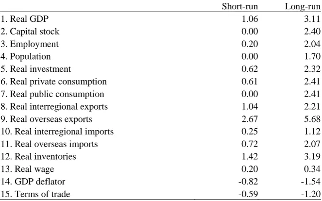
Tables 1 and 2 present short-run and long-run consequences for the LA County regional economy of a 1 per cent improvement in primary factor productivity in all industries other than dwellings services. Productivity improvement is chosen as an illustrative simulation because it is a supply-side shock. IMPLAN data is typically used for regional input/output impact assessments. Input/output analysis is not suitable for analysis of supply-side shocks.
The short-run and long-run labour market closures are as described in Section 2.2.1. In both the short-run and long-run, household consumption spending is assumed to be a fixed proportion of household income.
21
capital stocks endogenous. Long-run industry-specific investment is determined via an assumption of exogeneity in industry-specific gross capital growth rates.
In the short-run, regional and federal government real public consumption spending are exogenous. In the long-run, the ratio of regional and federal government real public consumption spending to real regional private consumption spending is exogenous.
4.2 Short-run consequences of a 1 per cent improvement in primary factor productivity
The shock is a 1 per cent improvement in the productivity of primary factors used in all Los Angeles County industries other than dwellings services. In the short-run, industry-specific capital stocks cannot adjust to the shock. Via equation (5), short-run employment is largely tied-down via the exogeneity of regional population. In the absence of any movement in regional factor employment, a 1 per cent primary factor productivity improvement should increase regional real GDP by 1 per cent (row 1, Table 1). However, with regional employment sticky via short-run exogeneity of regional population (row 4), the productivity improvement causes the regional real consumer wage to increase (row 13). Via equations (1) – (3) this induces small short-run increases in hours worked per worker, participation rates, and employment rates. This accounts for the small short-run increase in regional employment (row 3). The short-run increase in regional employment is responsible for real GDP increasing by more than the 1 percentage point attributable to productivity growth alone (row 1). With capital stocks fixed (row 2), but productivity and employment rising, rates of return on physical capital increase. This accounts for the short-run increase in real investment (row 4). Real private consumption is linked to real income. With real GDP higher (row 1) so too is real regional income. This accounts for the short-run increase in real private consumption spending (row 6). With regional economic activity higher than it would otherwise have been, so too are interregional and overseas imports (rows 10 and 11 respectively). Note that real public consumption spending is unchanged (row 7). As such, real GNE (rows 5 – 7) increases by less than real GDP (row 1). This requires the regional real balance of trade to move towards surplus. Hence, the increases in real regional exports (rows 8 and 9) exceed the increases in real regional imports (rows 10 and 11). Movement towards surplus in the real regional balance of trade requires the regional price level to fall relative to the external price level (row 14). The expansion in regional export volumes involves movement down fixed interregional and international export demand schedules. Hence regional export price fall. The expansion in foreign and inter-regional imports exerts slight upward pressure on regional import prices. Together, these regional trade price movements cause the regional terms of trade to decline relative to what they would otherwise have been (row 15). The decline in the regional terms of trade explains why the increase in real private consumption (row 6) is less than the increase in real regional GDP (row 1).
22
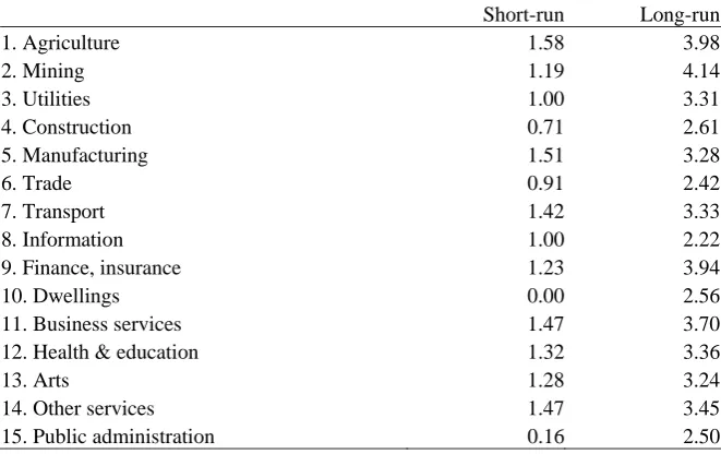
from the general increase in productivity experienced by all other sectors. Public administration (row 15) also experiences little output expansion. This reflects the exogeneity of aggregate real public consumption spending (Table 1, row 7). Prospects for the regional Construction sector (row 4) are largely determined by regional investment (row 5, Table 1). With regional real investment expanding by less than real GDP, the regional Construction sector is among the sectors experiencing the lowest expansion in output.
4.3 Long-run consequences of a 1 per cent improvement in primary factor productivity
Column 2 of Tables 1 and 2 report the long-run impacts on the LA County economy of improved primary factor productivity. In the long-run, the regional capital market closure is equivalent to an assumption that the regional economy can source as much capital as required at exogenously determined real rates of return. In the long-run, equation (4) is activated via exogenous determination of fPOP and endogenous determination of pop.
With very high values for αPOP, this is almost equivalent to an assumption that the regional economy can source as much labour as required at an exogenously determined real regional wage. However to reflect location preference, and some feedback to the national real wage from the regional economy, αPOP is set at a high, but not infinite, value9.
With exogenous regional rates of return, and near exogeneity of the regional real consumer wage, the increase in primary factor productivity generates sizeable long-run increases in employment of capital (row 2) and labour (row 3). However expansion of the long-run regional economy is limited by two factors. First, via equation (4), the regional real wage must rise to attract population from outside the region. This accounts for the long run increase in the LA County real wage (row 13). Second, expansion of the regional economy causes the regional terms of trade to decline (row 15) damping the potential increase in the values of the marginal product of capital and labour.
The increase in LA County primary factor productivity is projected to increase LA County real GDP by 3.1 per cent. Just under 1 percentage point of this increase is directly attributable to the rise in primary factor productivity. The remainder is due to increased employment of capital (row 2) and labour (row 3). The capital / labour ratio increases slightly (compare rows 2 and 3) because the long-run regional real wage must rise to attract population to the regional economy (row 13).
Long-run private consumption is assumed to be a fixed proportion of long-run regional income. Hence, with long-run real regional GDP higher, so too is regional private consumption (row 6). However expansion of the long-run regional economy is associated with import and export expansion (rows 8 – 11) and thus long-run terms of trade decline (row 15). This damps the increase in real (CPI-deflated) income relative to real GDP.
9 At present, α
POP is set at 5. In the future, we hope to set this parameter at values that reflect (i) the length
23
This explains why the increase in private consumption (row 5) is less than the increase in real GDP (row 1). The long-run ratio of public to private consumption spending is exogenous. Hence the long-run percentage change in public consumption spending (row 7) is the same as that for private consumption spending (row 6). Hence the increase in real public consumption spending is also less than the increase in real GDP. Long-run industry-specific investment / capital ratios are exogenous. This accounts for why the increase in aggregate real investment (row 5) is very similar to the increase in the aggregate capital stock (row 2). Since productivity growth is contributing about 1 percentage point to the increase in real GDP (row 1) the increase in the capital stock (row 2), and thus so too, investment (row 4), must be less than that of real GDP (row 1). Hence, with real investment, real private consumption, and real public consumption all rising by less than real GDP, the real balance of trade must move towards surplus (rows 8 – 11).
Table 1: Regional macro impacts (percentage change relative to basecase)
Short-run Long-run
1. Real GDP 1.06 3.11
2. Capital stock 0.00 2.40
3. Employment 0.20 2.04
4. Population 0.00 1.70
5. Real investment 0.62 2.32
6. Real private consumption 0.61 2.41
7. Real public consumption 0.00 2.41
8. Real interregional exports 1.04 2.21
9. Real overseas exports 2.67 5.68
10. Real interregional imports 0.25 1.12
11. Real overseas imports 0.72 2.07
12. Real inventories 1.42 3.19
13. Real wage 0.20 0.34
14. GDP deflator -0.82 -1.54
24
Table 2: Sectoral impacts (percentage change relative to basecase)
Short-run Long-run
1. Agriculture 1.58 3.98
2. Mining 1.19 4.14
3. Utilities 1.00 3.31
4. Construction 0.71 2.61
5. Manufacturing 1.51 3.28
6. Trade 0.91 2.42
7. Transport 1.42 3.33
8. Information 1.00 2.22
9. Finance, insurance 1.23 3.94
10. Dwellings 0.00 2.56
11. Business services 1.47 3.70
12. Health & education 1.32 3.36
13. Arts 1.28 3.24
14. Other services 1.47 3.45
15. Public administration 0.16 2.50
5 CONCLUSIONS
25
26
REFERENCES
Anderson, K. J.A. Giesecke and E. Valenzuela (2008) “How would global trade liberalization affect rural and regional incomes in Australia?” General Working Paper No. G-176, Centre of Policy Studies, Monash University, July 2008.
Dixon, P.B., B.R. Parmenter, J. Sutton and D.P. Vincent, 1982, ORANI: A multi-sectoral
model of the Australian economy, North-Holland, Amsterdam.
Dixon, P.B., B.R. Parmenter, A.A. Powell, P.J. Wilcoxen. 1992. Notes and problems in
applied general equilibrium economics. Advanced Textbooks in Economics.
North-Holland, Amsterdam, 1992.
Dixon, P.B. and M.T. Rimmer (2002). MONASH-USA: Creating a 1992 Benchmark Input-Output database. Centre of Policy Studies, Monash University, May, 2001 (revised June 2002).
Hanoch, G. (1971). CRESH Production Functions. Econometrica, vol 39, September, pp. 695 – 712.
Harrison, W. J. and K. R. Pearson, 1996, Computing Solutions for Large General Equilibrium Models using Gempack, Computational Economics, vol. 9, 83–127.
Horridge, J.M. , 2003, ORANI-G: A generic single country computable general
equilibrium model. <http://www.monash.edu.au/policy/ftp/oranig/oranig03.zip>
Madden, J.R. 1996. FEDERAL: A two-region multi-sectoral fiscal model of the Australian economy. In: Modelling and control of national and regional
economies: proceedings. Edited by Vlacic, L., et al. , 347-352. Oxford:
Pergamon.
Minnesota IMPLAN Group (1997) IMPLAN System (19xx/20xx data and software), 1725 Tower Drive west, Suite 140, Stillwater, MN 55082, www.implan.com, 1997.
Minnesota IMPLAN Group (2009) “Elements of the Social Accounting Matrix”. MIG IMPLAN Technical Report TR-98002.
United States International Trade Commission (2004), The Economic Effects of
Significant U.S. Import Restraints: Fourth Update 2004, Investigation No.
332-325, Publication 3701, June.
United States International Trade Commission (2007), The Economic Effects of
Significant U.S. Import Restraints: Fifth Update 2007, Investigation No. 332-325,
27