Modeling rejection immunity

(1)

R E S E A R C H

Open Access

Modeling rejection immunity

Andrea De Gaetano

1*

, Alice Matone

1

, Annamaria Agnes

2

, Pasquale Palumbo

1

,

Francesco Ria

3

and Sabina Magalini

2

*Correspondence: andrea. [email protected]

1_{CNR-IASI BioMatLab, UCSC Largo}

A. Gemelli 8, 00168 Rome, Italy Full list of author information is available at the end of the article

Abstract

Background: Transplantation is often the only way to treat a number of diseases leading to organ failure. To overcome rejection towards the transplanted organ (graft), immunosuppression therapies are used, which have considerable side-effects and expose patients to opportunistic infections. The development of a model to

complement the physician’s experience in specifying therapeutic regimens is therefore desirable. The present work proposes an Ordinary Differential Equations model accounting for immune cell proliferation in response to the sudden entry of graft antigens, through different activation mechanisms. The model considers the effect of a single immunosuppressive medication (e.g.cyclosporine), subject to first-order linear kinetics and acting by modifying, in a saturable concentration-dependent fashion, the proliferation coefficient. The latter has been determined experimentally. All other model parameter values have been set so as to reproduce reported state variable time-courses, and to maintain consistency with one another and with the experimentally derived proliferation coefficient.

Results: The proposed model substantially simplifies the chain of events potentially leading to organ rejection. It is however able to simulate quantitatively the time course of graft-related antigen and competent immunoreactive cell populations, showing the long-term alternative outcomes of rejection, tolerance or tolerance at a reduced functional tissue mass. In particular, the model shows that it may be difficult to attain tolerance at full tissue mass with acceptably low doses of a single immunosuppressant, in accord with clinical experience.

Conclusions: The introduced model is mathematically consistent with known physiology and can reproduce variations in immune status and allograft survival after transplantation. The model can be adapted to represent different therapeutic schemes and may offer useful indications for the optimization of therapy protocols in the transplanted patient.

Background

It is unfortunately not rare in medical practice that some diseases lead to organ failure, which may eventually require organ transplantation. The liver, the kidney and the heart are the most frequently transplanted organs. Diseases leading to organ transplantation span a wide spectrum of medical conditions: cancer, infections, autoimmune and degen-erative diseases. Transplantation into the recipient of a foreign organ (graft), even from an individual of the same species (allograft), if left to itself causes rejection, a strong response by the recipient’s immune system leading to irreversible damage of the graft. Depending

(2)

on the time-frame over which rejection occurs, “acute” rejections are differentiated from “chronic” ones. Acute rejection develops in the first few weeks or months after transplan-tation and is produced by cellular and molecular mechanisms, which may partially differ from those leading, over the course of many months or years, to chronic rejection.

After many decades of experimentation on animals and cells, and of the development of pharmacological tools, organ transplantation has evolved into a common therapeu-tic procedure. The success of a solid organ transplant relies in equal measure on the technical aspects of the implant and on the recipient’s acceptance or tolerance of the implanted graft. This last phenomenon is clinically induced by the administration of immunosuppressive drugs, which specifically decrease the recipient’s reactivity towards the graft, thus allowing the maintenance of the functional activity of the organ. Currently available drugs belong to several classes (calcineurine inhibitors (CNI), antimetabolites, target of rapamycin (TOR) inhibitors, steroids, and monoclonal antibodies) [1]. Canoni-cal combinations of these drugs are typiCanoni-cally used by the attending physician in a rather standardized fashion, attempting to maintain measurable drug plasma concentrations within established limits. Episodic and emergency use of immunosuppressive agents is then performed if signs of rejection become clinically evident.

Acute rejection response has been extensively studiedin vivoandin vitro. From avail-able studies, indications on the action of several drugs in controlling acute rejection and maintaining vitality of the graft have been obtained. However, even if the recipient initially accepts the graft, the more insidious and slow phenomenon of chronic rejection often ensues. The pathogenesis of chronic rejection is less well known and may depend not only on a partially different set of immune response mechanisms, but also on actual drug toxicity, recommending the use of the minimal clinically effective dose of medication.

(3)

drug efficacy, possible drug adverse effects and the development of immune tolerance or graft acceptance.

In the present work we propose a tentative mathematical model of the rejection towards a solid organ transplant (kidney, liver, pancreas, heart). This model describes the evolu-tion of the main cellular immune response as well as the kinetics and acevolu-tion of a single representative drug (e.g. cyclosporine). In order to have some physiological support for parameter assessment, a Mixed Lymphocyte Reaction (MLR) experiment was performed, on the basis of which the clonal expansion rate of T-cells could be determined. This experiment was chosen because the parameter of interest for the model was directly computable from the experimental data. Simulations with Matlab©2010b have been per-formed and, on the basis of the experimentally determined clonal expansion rate and of relevant published material, the other model parameters were calibrated. While the cur-rent model is relatively simple, it introduces the main elements needed for the eventual description of more detailed response dynamics. Three case scenarios are discussed: non-immunosuppressed transplantation and two immunosuppressive therapeutical regimens, one with moderate drug dose and the other with high drug dose. Additional simulations were made in order to explore different hypothetical therapy scenarios. Also, three state variables were selected as being most clinically relevant, and a sensitivity analysis was performed on these at two time points (one and ten years post-transplant).

Methods

Relevant physiology

After transplantation, the majority of exogenous molecules on the allograft are recog-nized by the immune system as self-antigens, as they are the same in both the donor and recipient. The main donor molecules which induce the immune response are those coded from the Major Histocompatibility Complex (MHC) genomic locus, which is the most polymorphic one on the human genome (it is essentially impossible to find two per-sons with the same gene cluster, except for monozygotic twins). Proteins coded by the MHC are located on the cell surface and bind antigen epitopes, creating a complex, which is recognized by the T-Cell Receptor (TCR) on T-lymphocytes, inducing the immune response. Cells which carry the MHC/epitope complexes are called Antigen Presenting Cells (APCs) [9].

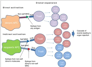
In the conventional immune response, self-APCs carry external antigen epitopes bound to self-MHC molecules. APCs normally circulate in the body and are found in every organ - during transplantation many APCs from the donor are introduced in the recipient, and they carry the donor’s MHCs. In fact, MHCs on donor cells are the major target of the rejection immune response [10], as T-cells can recognize complexes formed by allogenic MHCs [11]. This mechanism is called “direct activation”, since there is no processing of the antigen, and it is faster than the indirect activation, where recipient’s APCs have to process donor’s antigen [12]. In Figure 1 a schematic representation of the direct and indirect mechanisms is shown.

(4)

donor’s APC

recipient’s APC

T-cell T-cell T-cell

T-cell clone

T-cell clone T-cell clone

T-cell clone

T-cell clone T-cell clone T-cell clone

T-cell clone T-cell

clone

T-cell clone

Cascade of events leading to organ rejection

D i r e c t a c t i v a t i o n

Self MHC

I n d i r e c t a c t i v a t i o n

Self MHC Non-self MHC

TCR

Epitope from donor’s non-self MHC

Epitope from any antigen

Epitope from non-self donor’s molecules

C l o n a l e x p a n s i o n

Figure 1 Direct and indirect activation mechanisms.With the direct activation mechanism the donor’s Antigen Presenting Cell, expressing its MHC molecule (red) and carrying a general epitope (green), is recognized from the T-Cell Receptor and activates T-cell clonal expansion. In this case it is the actual MHC molecule which is recognized as non-self from the TCR. In the lower part of the figure, the two possible indirect activation scenarios: self APC, expressing self MHCs, can present an epitope from graft antigens recognized as non-self (blue) or from donor’s MHC (red).

“Alloreactive T-lymphocytes are[in any case]requisite mediators of allograft rejection” [11].

At the level of detail used in the present work, CD4+ and CD8+ T-lymphocytes (“helper” and “cytotoxic”) are not distinguished, and we consider them together as T-cells mediating rejection. The reasons for this simplification are that both T-cell types increase in number during the immune response and that they can both be activated by exogenous antigens. It has recently been shown that both class I and II MHC molecules (respectively recognized by CD4+ and CD8+ T-cells) can bind extracellular antigens (“cross priming”), while it was previously thought that class I MHCs could only present intracellular anti-gen [14]. In the course of direct activation, APCs are either destroyed or will eventually undergo apoptosis. Since donor’s APCs do not reproduce in the allograft, direct T-cell activation is a time-limited process. The immune response, however, does not terminate since there is continuous supply of donor-specific molecules, produced from the con-stantly proliferating cells in the graft. T-lymphocyte activation occurs as long as the graft is present in the recipient.

(5)

the number of directly activated T-cells is larger than the number of indirectly-activated T-cells, the latter constituting less than 10 percent of the total cellular alloimmune repertoire [15].

Two aspects of graft rejection have not been explicitly included in the model for sim-plicity. The first is the increased production of lymphocytes from lymphoid organs, which receive various signals from stimulating molecules (cytokines). This mechanism has been shown [16] to take place when an inflammatory process (i.e.rejection) is ongo-ing. The second aspect of rejection is the appearance of the graft-versus-host disease, where donor’s T-cells present in the allograft react towards recipient’s antigens. This last phenomenon depends on the type of the transplanted organ and may be negligible in most cases of solid organ transplantation.

MLR is an in vitroexperiment used to study alloreactive T-cells response to exoge-nous MHC molecules: it is used in clinical practice as a prediction rejection test before performing organ transplantation. MLR is induced growing mononuclear cells of an individual with those of another individual, these cells being isolated from

periph-eral blood: the difference between MHC loci of the two individuals induces clonal

expansion of alloreactive lymphocytes [17]. One of the model parameters, the one corresponding to the clonal expansion rate of T-cells, was determined by an MLR experiment.

In the present model we consider one of the most frequently used immunosuppression therapy protocols, based on calcineurine inhibitors (e.g. cyclosporine)[1], which block T-cell clonal expansion. Drugs of this class inhibit signal transduction when TCRs rec-ognize the epitope, so that the cell does not proliferate even when activated. Other types of therapy, acting through different mechanisms, could also be considered, extending the present approach.

The model

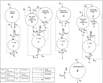
The model is represented in block diagram form in Figure 2, showing all compartments and the relative dynamics. Organ transplantation is assumed to occur at timetτ in the

life of the patient. Before transplantation, the major components of the immune system involved in transplant rejection are assumed to be at equilibrium. The choice of the time

t0, at which simulations begin, is therefore irrelevant, as long as t0 < tτ. In order to

represent organ damage, we assume that antigen is released into the blood stream propor-tionally with the viable mass of the corresponding tissue, and consequently that the viable graft mass is proportional to bloodstream antigen mass, so that a substantial decrease in antigen concentration will indicate organ failure.

With the transplantation of an allograft at timet=tτ, the state of the immune system

(6)

kxf T – cells

Ce

kuτ

Cyclosporine F General Antigen E kf kxu kxl kxc kcac(F) kxuc kxlc NRep graft antigen DPsn U ke

kxe kxec

Nrep graft antigen IPsn

Prc

Z

kxzkxzc Nrep - NPrc

graft antigen IPsn

Y kyτ

kzy kxy ks Rep graft antigen Ipsn Prc L NPrc Non Processed Prc Processed DPsn Direct Presentation IPsn Indirect Presentation NRep Non Reproducing Rep Reproducing

Rep - NPrc graft antigen IPsn

S ksτ

kls

kxsc

kxyc

T – cells

Cl kxcl kxce kxc kxcs kc kcac(F)

§

kc kcac(F)

§

T – cells

Cu kxc kxcu kc kcac(F)

§

T – cells

Cl kcac(F)

§

kxc kxcy kxcz kc S* mass movement stimulation inhibition

Figure 2 Model block diagram.State variables are represented with circles, the above ones for the different antigen types, the bottom ones for specific T-cells. On the bottom right the pharmaceutical dynamics is represented, the symbol§indicates the site of action of the drug. Solid arrows represent mass transfers, while dashed lines indicate stimulation and inhibition (arrow end and dot end, respectively).

State variables are generally defined in terms of concentrations, and we suppose a single vast plasma/interstitial fluid volume space where, given time, all species distribute. State variables and parameters, with corresponding units of measurement, are listed in Tables 1 and 2, respectively.

(7)

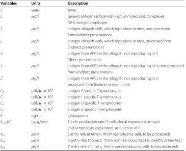
Table 1 Model variables

Variables Units Description

t years time

E μg/l generic antigen (antigenically active molecules): complexes MHC-antigenic epitopes

S μg/l antigen allograft cells, which reproduce in time, non-processed form(indirect presentation)

L μg/l antigen allograft cells, which reproduce in time, processed form (indirect presentation)

U μg/l antigen from APCs in the allograft, not reproducing in it

(direct presentation)

Y μg/l antigen from APCs in the allograft, not reproducing in it, non-processed form (indirect presentation)

Z μg/l antigen from APCs in the allograft, not reproducing in it,

processed form (indirect presentation) Ce cell/μl×103 antigenEspecific T-lymphocytes Cl cell/μl×103 antigenLspecific T-lymphocytes Cu cell/μl×103 antigenUspecific T-lymphocytes

Cz cell/μl_×103 _antigen_Z_{specific T-lymphocytes}

F ng/ml cyclosporine

kcac(F) l/μg/year T-cells production rate (T-cells clonal expansion), antigen and lymphocyte dependent, as function ofF

ksτ μg/l Sentry rate at timetτ(from reproducing cells, to be processed)

kuτ μg/l Uentry rate at timetτ(from non-reproducing cells, directly presented)

kyτ μg/l Yentry rate at timetτ(from non-reproducing cells, to be processed)

T-cells. The processing mechanism is represented in the same way as for antigensSand

L. The model is detailed in the following equations:

dE

dt =ke−kxecCeE−kxeE, E(0)=E0 (1)

dCe

dt =kc+kcac(F)CeE−kxceECe−kxcCe, Ce(0)=Ce0 (2) dS

dt =ksτ+ksS

1− S

S∗

−kxscClS, S(0)=0 (3)

dL

dt =klsS−kxlcClL−kxlL, L(0)=L0 (4) dCl

dt =kc+kcac(F)ClL−kxcsSCl

−kxclLCl−kxcCl, Cl(0)=Cl0 (5)

dU

dt =kuτ−kxucCuU−kxuU, U(0)=U0 (6) dCu

dt =kc+kcac(F)CuU−kxcuUCu−kxcCu, Cu(0)=Cu0 (7) dY

dt =kyτ−kxycCzY−kxyY, Y(0)=Y0 (8) dZ

(8)

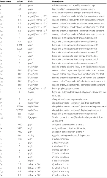
Table 2 Model parameters

Paramaters Value Units Description

t0 35 years minimum time considered by system, in days

tτ 40 years time in which transplantation occurs, in days

ke 1 μg/l/year constant environment antigen entry into the body

kxec 1.5 μl/cell/year×10−3 second orderCdependentEelimination rate constant kxsc 0.15 μl/cell/year×10−3 second orderCdependentSelimination rate constant kxlc 0.7 μl/cell/year×10−3 second orderCdependentLelimination rate constant kxuc 0.5 μl/cell/year×10−3 second orderCdependentUelimination rate constant

kxyc 0.5 μl/cell/year×10−3 second orderCdependentYelimination rate constant kxzc 1 μl/cell/year×10−3 second orderCdependentZelimination rate constant

kxe 1 year−1 first order elimination rate from compartmentE

kxl 0.7 year−1 first order elimination rate from compartmentL

kxu 0.001 year−1 first order elimination rate from compartmentU

kxy 0.001 year−1 first order elimination rate from compartmentY

kxz 1 year−1 first order elimination rate from compartmentZ

kls 1.5 year−1 first order transfer rate from compartmentStoL

kzy 6 year−1 first order transfer rate from compartmentYtoZ

kxc 1 year−1 first order elimination rate from compartmentC

kxce 1 l/μg/year second orderEdependentCeelimination rate constant kxcs 0.02 l/μg/year second orderSdependentClelimination rate constant kxcl 0.02 l/μg/year second orderLdependentClelimination rate constant kxcu 0.02 l/μg/year second orderUdependentCuelimination rate constant

kxcy 0.02 l/μg/year second orderYdependentCzelimination rate constant kxcz 0.02 l/μg/year second order Z dependentCzelimination rate constant kc 0.3 cell/μl/year×103 basal lymphocyte production

ks 2 1/year first order S dependent S production and elimination rate

constant

S∗ 7 μg/l allograft maximum regeneration rate

κf 0 ng/ml/year drug delivery rate - scenario 1 (no drug treatment)

κf 36500 ng/ml/year drug delivery rate - scenario 2 (moderate drug treatment) κf 127750 ng/ml/year drug delivery rate - scenario 3 (high drug treatment)

kxf 365 1/year first order elimination rate from compartment F

kcacF 2.92 l/μg/year T-cells production rate (T-cells clonal expansion), A and c dependent

Sτ 1000 μg/l antigen S concentration at timetτ

Uτ 1000 μg/l antigen U concentration at timetτ

Yτ 1000 μg/l antigen Y concentration at timetτ

λ 0.01 ml/ng kcacdecreasing coefficient, F dependent

E0 1.38 μg/l Einitial condition

S0 0 μg/l Sinitial condition

L0 0 μg/l Linitial condition

U0 0 μg/l Uinitial condition

Y0 0 μg/l Yinitial condition

Z0 0 μg/l Zinitial condition

F0 0 ng/ml Finitial condition

Ce0 1.1 cell/μl×103 CEvalue att=t0

Cl0 0.3 cell/μl×103 CLvalue att=t0

Cu0 0.3 cell/μl×103 CUvalue att=t0

(9)

dCz

dt =kc+kcac(F)CzZ−kxcyYCz

−kxczZCz−kxcCz, Cz(0)=Cz0 (10)

dF

dt =kf −kxfF+ κ_f kxf

δ(t−tτ), F(0)=0 (11)

ksτ =δ(t−tτ)Sτ (12)

kuτ =δ(t−tτ)Uτ (13)

kyτ =δ(t−tτ)Yτ (14)

kf =

0, if t≤tτ

κ_f, if t> tτ

(15)

kcac(F)= kcacFe−λF (16)

In equation 1, describing antigen E dynamics, the rate ke represents the entry of environmental antigens into the body, assumed to be constant throughout the con-sidered period of time (before as well as after transplantation). The elimination terms

kxecandkxe describe antigen neutralization due respectively to cell action and to T-cell-independent elimination of the antigen (as it happens e.g. through chemical and physical elimination mechanisms, such as lipases, mucus secreted by respiratory and gastrointestinal tracts etc.).

Equation 2 represents the dynamics of T-lymphocytes which react towards antigen

E:kcindicates constant physiological T-lymphocyte production from lymphoid organs,

kcac(F)ECerepresents T-cell clonal expansion after antigen contact, which is inhibited by drug action, by setting the ratekcacF as a proper function of the drug concentration

F. T-lymphocytes are also “consumed” by antigen, in the sense that upon T-cell inter-action with antigen, the lymphocyte eventually undergoes apoptosis (programmed cell death): this is described by the elimination termkxceECe. We introduced another elim-ination term,kxcCe: lymphocytes die for apoptosis even if they do not encounter any antigen after a certain period, and we assume this mechanism to be proportional to T-cell concentration.

The regenerating antigen is described by equation 3: at timetτ there is an impulsive

entry, modeled by a Dirac delta (Eq. 12). Once the organ is transplanted, its cells regener-ate: the growth rate is assumed to be logistic of parameterks, limited by a carrying capacity

S∗, so thatSconcentration tends towardsS∗, whether it is above or below it. The elimina-tion termkxscClS, depends onSconcentration and on T-cells primed from the processed form of the antigen. The non-processed form is not ready to activate T-lymphocytes, but it is destroyed by T-cells activated from the processed form. In fact, T-cells activated from the processed antigen (C_l) are primed to react against cells carrying the same epitopes (graft cells). Organ rejection is thus represented by theSantigen elimination, this being related to organ mass.

The processed form of the regenerating antigen is described by equation 4, where the only positive entry is represented by the termklsSdepending on the unprocessed antigen concentration; the two elimination terms are similar to those in the previous described equations, representing lymphocyte-dependent and -independent elimination, respec-tively. Equation 5 describes theC_l lymphocyte dynamics, with the constant entry, the

(10)

with both antigens S and L, and antigen-independent elimination. The directly pre-sented antigenUis represented by equation 6: a Dirac’s delta describes impulsive entry at transplantation time, while elimination happens in two ways, dependent and inde-pendent from T-cells, respectively. U-specific T-lymphocytes, Cu, are represented in equation 7, including constant production rate, clonal expansion, antigen-dependent and independent elimination.

The last three equations represent the non-regenerating antigen which has to be pro-cessed, its non-processed form (Y), the processed form (Z) andZ-specific T-cells. The dynamics are similar to theS,LandClsubsystem, the only difference being that this anti-gen does not reanti-generate. Equation 8 has an impulsive entry and elimination dependent and independent from T-lymphocytes; in equation 9 the entry depends onY concentra-tion, and the usual two elimination terms follow; equation 10 is similar to equation 5. Equations 12, 13 and 14 describe the impulsive antigen entries into the system. In each case an antigen concentration (respectively Sτ, Uτ and Yτ) is multiplied by a Dirac

delta term acting at time tτ. The end result is the representation of the appropriate

instantaneous change inS,UandYcompartments at the time of transplantation. Finally, immunosuppressor pharmacokinetics is described by equation 11. For the pur-pose of the present model, given the long time-scale considered, drug administration is assumed to be continuous, with average ratekf (equation 15) of delivery into the circu-lation. The drug is eliminated from the circulation following a linear, first-order process with rate constantkxf. Since before transplantation no treatment is administered,kf is 0 before timetτ, while it is equal toκf from the time at which therapy begins, which we assume to betτ. The term

κf

kxfδ(t−tτ)represents therefore the (impulsive) loading dose

of the drug, necessary to bring it instantaneously to the equilibrium level, at which it is constant thereafter. After antigen contact, T-cells would spontaneously give rise to a (fast) clonal expansion. The immunosuppressive effect of the drug, leading to a slower increase of T-lymphocyte concentrations, is described by the exponential decrease in the clonal expansion coefficientkcacF produced by proportionally increasing drug concentrationsF (with effect rate constantλ): this is represented by equation 16. The drug is in fact thought to block signal transduction after antigen contact, in a concentration-dependent fashion, thus disabling clonal expansion and reducing T-cell proliferation. Equation 11 represents the pharmacokinetics of the anti-rejection drugFwith given constant entry (depending on the administration scheme), linear elimination and with impulsive entry assumed to be simultaneous with transplantation. Equations 12-16 and Tables 1 and 2 define each sym-bol used. Tables 1 and 2 also report units of measurement for all variables and parameters.

Model parameters

(11)

Mixed lymphocyte reaction

Blood samples were collected from four healthy donors and peripheral blood mononu-clear cells (PBMCs), from three of the blood samples, were stained with the lipophilic fluorescent molecule Carboxyfluorescein Succinimidyl ester CFSE. The CellTrace CFSE Cell Proliferation Kit (Invitrogen) was used following the protocol provided by the

man-ufacturer. Cells were stained with PBS/5%FCS/CFSE-50 μM for ten minutes at room

temperature and then washed twice. Non-labeled PBMCs obtained from the fourth healthy donor were used as allogenic stimuli and labeled PBMC were cultured in vitro in the presence or absence of non-labeled PBMC with a ratio of 2:1 (2×107 labeled PBMC versus 107 non-labeled PBMC). Three days later, cells were harvested and stained with PE-conjugated anti-CD3 mAb (Becton Dickinson). Cells were then analyzed at cytofluorimeter FACS-calibur (Becton Dickinson) and data were acquired by the software CellQuest pro.

Parameter computation

Since lymphocytes were exposed to a large amount of allogenic cells, we assume that the experiment reflects the maximal clonal expansion that can be achieved at a “maximal” antigen concentration. From equations 2, 5, 7 and 10,kcacF dimensions are l/μg/year. From the experiment we measured the percentage of replicating cells per day, which has to be divided by the maximal antigen concentration expressed asμg/l. The concentra-tion of MHC molecules in the experimental preparaconcentra-tion was approximated as follows. On a cell surface there are approximately 105MHC molecules, and there were approx-imately 106_{cells/ml of blood. It thus follows that the concentration of MHC molecules} was 105×106/ml,i.e.1014molecules per liter. Considering both MHC class I and class II molecules, the average molecular weight is approximately 60 kDa, meaning that one

mole of MHC weights 60×103grams. Since in one mole there is one Number of

Avo-gadro of molecules, 1014molecules correspond to 1014/(6×1023)moles, or approximately

(1018 × 6)/(1023 ×6))g/l. The parameter kcacF has therefore been computed as the clonal expansion per day divided by the maximal antigen concentration (10−5 _{g/l or} 10μg/l), afterwards multiplied by 365 days. No formal statistical parameter estimation (e.g.Maximum Likelihood-based) was attempted. In keeping with the generally qualita-tive character of this model’s predictions, the desired outcome of the MLR experiment was an indicative, plausible value for the rate of clonal expansion, and, as is apparent, this plausible value itself is conditional onad-hocassumptions (e.g.that maximal stimulation is equivalent to an antigen concentration of 10μg/l).

Results

Clonal expansion rate from MLR

(12)

Figure 3 Cytofluorimeter analysis.Cells were analyzed for CD3 expression and CFSE incorporation. T-cells are selected with CD3+ marker, on the y axis the group of cells above the horizontal line are CD3+. On the x axis, the amount of CFSE indicates if cells replicated or not: for each cell division the amount of CFSE incorporated in DNA is reduced by half. The upper left panel (red circle) contains T-cells which have replicated.

So, for every 100 cells in the final count, on day 1 we have 76.5 (cells that did not replicate) + 3 (cells that replicated), that is 79.5% of the final 100%. The global replication rate at each rate was computed solving the following equation:

y3=y0e−kmaxt (17)

wherey0is the total number of cells on day 0 (approximately 79) andy3is the number of total cells on day 3 (100), whilekmaxis the replication rate. Solving (17) witht=3 we obtainkmax=0.08/day.kcacF =0.08/10−5l/g/day, which is 2.92l/μg/year.

Model simulation

The model has been implemented in Matlab©2010b, and simulations are presented showing the behavior of the several types of antigen and corresponding specific T-cell populations after transplantation of a solid organ. Three scenarios are depicted, corresponding respectively to the no-therapy, moderate therapy and maximal therapy sit-uations. A time range from 35 to 60 years is shown, hypothesizing that transplantation occurs at time 40 years.

In Figure 4 all antigen types, the corresponding T-cell dynamics, and drug concentra-tions, are shown in the three therapy cases; subfigure 4.1 shows drug dynamics. In all subfigures the solid line (–) represents the no-therapy case, the dashed line (- -) refers to the moderate drug dose while the dotted line (..) refers to the high drug dose. Vari-able concentration ranges, as will be explained in the discussion, are in agreement with physiological limits.

Concentrations are assumed to be constant if no traumatic events happen during life. As the allograft is introduced (taking,e.g., tτ = 40 years), all antigen types described

(13)

40 50 60 0 200 400 4.1 Pharmaceutical years

F − ng/ml

40 50 60

0 0.5 1

4.2 Antigen E

years

E − microg/l

40 50 60

0 1 2 3

4.3 T−Lymphocytes C

E

years CE

− cell/microl x10

3

40 50 60

0 5 10

4.4 Antigen S

years

S − microg/l

40 50 60

0 5 10

4.5 Antigen L

years

L − microg/l

40 50 60

0 10 20

L

years CL

− cell/microl x10

3

40 50 60

0 5 10

4.7 Antigen U

years

U − microg/l

40 50 60

0 50

U

years CU

− cell/microl x10

3

40 50 60

0 5 10

4.9 Antigen Y

years

Y − microg/l

40 50 60

0 10 20 30

4.10 Antigen Z

years

Z − microg/l

40 50 60

0 50

Z

years CZ

− cell/microl x10

3

Figure 4 Variables dynamics plots.For each variable three scenarios are shown: solid line represents no therapy administration, the dashed line a middle immunosuppressant dose, and the dotted line a high dose. In Figure 4.1 the pharmaceutical dynamics is shown, while in the other plots each antigen dynamics is in line with the respective T-cell plot .

transplantation), as antigen from the organ is continuously produced and never vanishes (T-lymphocytesCl, Figure 4.6). If no therapy is applied, T-cell levels remain high and will bring the organ to a minimal size (rejection and failure): as can be noticed, the continuous line in the regenerating antigen graph (concentration of antigensSandL, Figure 4.4 and 4.5) is very low.

The dashed line represents the case in which administration of a moderate amount of immunosuppressive drug (such as cyclosporine) takes place. We assume that the drug is given simultaneously with the organ transplantation and that the patient is continuously and constantly treated (subfigure 4.1). It should be noticed that, as the increase of T-cell concentration is much lower, antigen level remains higher than the no-therapy case. This indicates that the graft is not totally destroyed by the immune system.

(14)

SubFigures 4.2 to 4.11 show the time course of specific antigens and their respective T-cell dynamics. In subFigures 4.2 and 4.3, generic antigen and generic T-lymphocyte concentrations are reported. If no therapy is administered, these dynamics are at equilib-rium. With therapy, generic T-cell concentration decreases (depending on drug dose): this indicates that immunosuppression is not specific in lowering T-cell expansion towards the graft. Instead, it reduces proliferation of all T-cells and, as a consequence, environmental antigen permanence levels in the body (E) increase.

In subfigures 4.4, 4.5 and 4.6, the concentrations of regenerating antigen in the non-processed (S) and processed (L) forms, as well as T-cells that respond to it (Cl), are shown. As seen before, in the absence of therapy, low antigen and high T-cell levels are reached after transplantation, while with drug administration antigen and T-cell concentrations are respectively higher and lower. This is the only case in which antigen never goes to zero because it is produced from regenerating graft cells. Dynamics of directly presented, non-regenerating antigen (U) and corresponding T-cells (Cu) are shown in subfigures 4.7 and 4.8: without therapy T-cells rapidly expand and consequently the antigen is rapidly elim-inated, while, with therapy, the action of T-cells is less aggressive on this type of antigen, which will eventually be eliminated because it does not regenerate. The non-regenerating and indirectly presented antigen (subFigures 4.9 and 4.10) has to be processed: there is a delay in the increase ofZ, which depends on non-processed antigen (Y) dynamics. The unprocessed antigen rapidly grows and rapidly vanishes as it is processed to the indirectly presented form and is no longer produced (because it derives from APCs not reproducing in the graft).

In subfigure 4.11 the dynamics of specific T-cells primed for antigenYandZis shown. In this case as well, as drug dosages increase, T-cell concentrations decrease and antigen levels rise.

From the graphs shown it is evident that is not easy to find the right drug dosage. In fact, it can be seen that when the dose is moderate T-cell levels are adequate but the graft tissue size is too small, while, as drug concentrations increase, T-lymphocyte levels are not sufficient to defend the patient from infections. The perfect situation would be to find a therapy level, which is effective in saving the graft from rejection, but does not unduly expose the individual to infections.

Effect of immunosuppression on T-cell reaction towards infection

In order to explore the predictive ability of the model, a simulation of an infection occur-ring two years after transplantation has been performed: the environmental antigenEand its specific T-cell population are shown in Figure 5. It is clear that, if the patient is not under treatment with the immunopuppressor (solid line) the immune system reacts nor-mally (big increase in T-lymphocyte concentration) and the antigen is quickly brought back to equilibrium levels. If the subject is immunosuppressed, T-cell population growth is inhibited in a drug-dosage-dependent fashion, and the patient is not able to fight the infection (elevatedEantigen levels maintained for a long time).

Balance between organ survival and immunosuppression

(15)

39 40 41 42 43 44 45 0

5 10 15

1.Environmental Antigen

years

E − microg/l

39 40 41 42 43 44 45

0 5 10 15

2.T−Lymphocytes − C

E

years CE

− cell/microl x10

3

Figure 5 Environmental antigen and lymphocytes reaction to infection with different drug dosages. Solid line, no immunosuppression; dashed line, middle dose; dotted line, high dose.

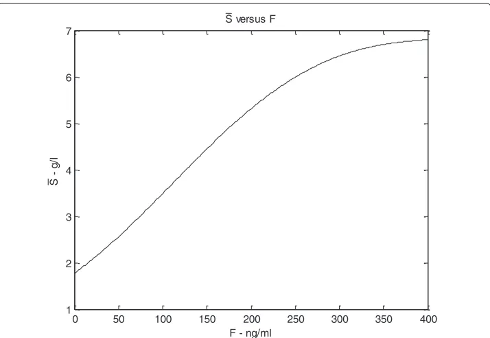
the patient has no actual exogenous organ mass. According to a proper setting of the model parameters (see the Appendix for more details), this equilibrium point is shown to be stable with respect to perturbations ofLandCl, and to be unstable with respect to perturbations ofS. On the other hand, the other, asymptotically stable equilibrium point corresponds to a non-elementary solution for the three state variables and is eventually reached after transplantation, when antigen and T-cells dynamics, under a certain drug dose, are balanced. Let us denote byS¯the value ofSat the stable equilibrium that is even-tually reached after transplantation, which represents the carrying capacity for antigen concentration (which we assume proportional to organ mass), as explained in subsection 3.2. A simulation is performed to show howS¯ changes in relation to varying immuno-suppressant concentrations. The plot in Figure 6 shows how the value ofS¯ varies with increasing drug doses: atF equal 0,S¯ has a positive (non zero) value, which is physio-logically plausible as the antigen would not be completely eliminated without drug, but its concentration would be low. As drug concentrations increase,S¯increases following a saturation curve: at high drug levels, when lymphocytes are inhibited, the antigen equi-librium approximates its maximum level. Similar diagrams are reported in Figures 7, 8, 9, 10 (see Appendix).

Hypothetical cyclical therapy

(16)

0 50 100 150 200 250 300 350 400 1

2 3 4 5 6 7

S versus F

F - ng/ml

S

g

/l

Figure 6S¯versusF. With increasing drug dose (x axis) theScarrying capacity, representing organ regeneration rate, increases and shows a saturation curve.

administration of immunosuppressant. The period of interruption equals the period of treatment, and the given dose is the same in each treatment period. A comparison between continuous and cyclical therapies is shown in Figure 11. The time interval applied in the simulation shown is one year; several other time intervals were tested (1 week, 2, 3, 4, 6 months, 2 years) and results were similar (results not shown). As shown in Figure 11.1, the immunosuppressant is given at one year intervals. The red line repre-sents the continuous therapy (low dose), while the blue and green lines the intermittent therapies (low and high doses). In Figures 11.2 and 11.3 the effect of the three therapy schemes on the environmental antigen (E) and the respective T-cells (Ce) are shown.

(17)

Figure 8 Bifurcation diagram forS, the antigen produced by graft cells, non-processed form.The bifurcation diagrams refer to the equilibrium points ofSin (19), according to varying amount of drugF(the bifurcation parameter) from 0 to 350 ng/ml. The continuous line indicates asymptotically stability, the dashed line indicates instability.

Figures 11.4, 11.5 and 11.6 show the dynamics of antigen S and its processed form

L- representing the organ mass - and the corresponding T-lymphocytes (Cl). The low intermittent dosage is less aggressive towards T-lymphocytes and, correspondingly, the subject is better protected against environmental antigens, but the organ is not protected from rejection as much as with the continuous dosage. The high intermittent dosage is less effective than the low continuous one, T-cells are not sufficiently inhibited and the graft antigen level is low.

Sensitivity analysis

Three variables have been identified as the most important ones to describe rejection

and immunosuppression in a clinical setting: S and T, representing the organ mass

(non-processed and processed form of the organ antigen) andCe, the T-cells specific for

(18)

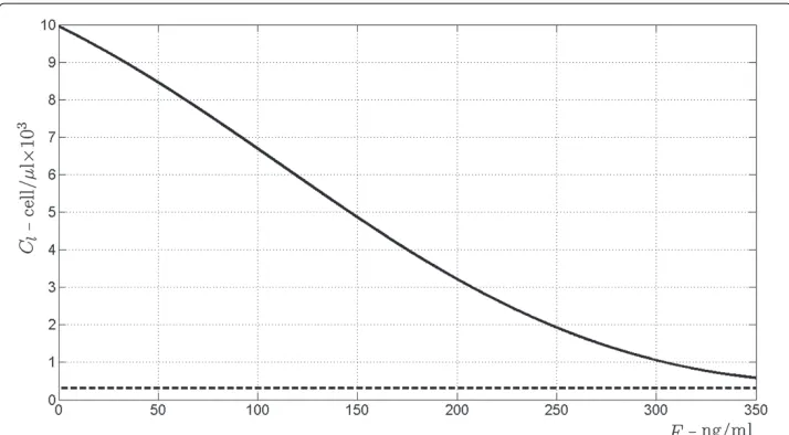
Figure 10 Bifurcation diagram forCl, T-cells activated from the processed antigen.The bifurcation diagrams refer to the equilibrium points ofClin (19), according to varying amount of drugF(the bifurcation parameter) from 0 to 350 ng/ml. The continuous line indicates asymptotically stability, the dashed line indicates instability.

the environmental antigen. Sensitivity analysis of these variables at 1 year and at 10 years after transplantation (t=41 andt=50) has been performed (tornado plots are shown in Figure 12).

Ceatt =41 andCeatt =50 plots are reported in Figures 12.1 and 12.2, respectively. The first observation is that the parameters affecting the two targets are the same, but in a different priority order. Also, at one year after transplantation, the variableCeis gener-ally more sensitive to parameter variations compared to the (near) equilibrium state at 10

(19)

-2 -1.5 -1 -0.5 0 0.5 1 1.5 kxcs kxcl kxcu kxcy kxcz S* ks kxsc kxl kxlc kls kxuc kxu kxyc kxy kxzc kxz kzy kxe lambda kxf kxec kc kxce ke kcacF kxc parm et ers

variable variation due to 1% increase of the parameter [cell/microl*103_]

12.1 - Ce, t=41

-1.5 -1 -0.5 0 0.5 1

kxcs kxcl kxcu kxcy kxcz S* ks kxsc kxl kxlc kls kxuc kxu kxyc kxy kxzc kxz kzy kxec kxe ke kxce lambda kxf kcacF kc kxc parm et ers

12.2 - Ce, t=50

-0.5 -0.25 0 0.25 0.5 0.75

ke kxec kxe kxce kxcu kxcy kxcz kxuc kxu kxyc kxy kxzc kxz kzy ks kxcl kxcs kxl kxlc kc kxc kxsc kls lambda kxf kcacF S* par m e te rs

12.3 - S, t=41

-0.75 -0.5 -0.25 0 0.25 0.5

ke kxec kxe kxce kxcu kxcy kxcz kxuc kxu kxyc kxy kxzc kxz kzy kxcl kc kxcs kxl kxlc S* kxsc ks kxc kls kxf kcacF lambda par m e te rs

12.4 - S, t=50

-2 -1.5 -1 -0.5 0 0.5 1 1.5 2

ke kxec kxe kxce kxcu kxcy kxcz kxuc kxu kxyc kxy kxzc kxz kzy kxcl kxsc kxcs kxl ks S* kxlc kc kxc kls kxf kcacF lambda parm et ers

12.5 - L, t=41

-1.5 -1 -0.5 0 0.5 1 1.5

ke kxec kxe kxce kxcu kxcy kxcz kxuc kxu kxyc kxy kxzc kxz kzy kxl kxlc kls kxcl kc kxsc ks S* kxcs kxc kxf kcacF lambda parm et ers

12.6 - L, t=50

(20)

years post-transplantation. Thekxcparameter is most influent on both variables: it rep-resents physiological T-cell elimination, due to natural apoptosis. It is noticeable that the other elimination rate,kxce, which is the elimination due to T-cell interaction with the antigen, is much lower. This is understandable, sincekxcrepresents a general mechanism that involves all cells whilekxceonly applies to cells in contact with their specific antigen. Another aspect worth noticing is that the rates which directly influence the environmen-tal antigen (E),kxe,kxecandke, are important att=41 but negligible att =50 (variation 0.05% or less).

Figures 12.3 and 12.4 show tornado plots forSatt=41 andSatt=50. The parameters, to which the two targets for the S antigen are most sensitive, are broadly the same. The major difference is in antigen regeneration. For botht=41 andt=50 variations inS∗are relevant, whereas variations inksonly impact model-predictedSlevels at 10 years post-transplantation, likely due to an accumulated effect of the small rate change. Besides the above described parameters, which regulate theSregeneration term, the parameters to which the variableSis most sensitive are the ones which regulate drug action on T-cells (kxf inverse correlation withSincrease, and lambda direct correlation withSincrease) and the T-cell clonal expansion rate (kcacF). Also the transfer rate fromS to Lantigen forms (kls) is a relevant parameter. It must be kept in mind thatS is the non-processed form of the regenerating antigen, and it does not directly activate T-lymphocytes, while it is directly eliminated by them. In fact, the parameters governing the variation ofL, the antigen processed form, are somewhat influent on both targets.

Tornado plots forL att =41 andL att =50 are reported in Figures 12.5 and 12.6, respectively. The processed form of the regenerating antigen is mostly affected by varia-tions of the parameters lambda,kcacF andkxf, as described above for the non-processed form, while it is not much affected by those parameters which regulate the processed form ofS(S∗andks), both at time 41 and 50. One interesting observation concerns the sensi-tivity to the parameterk_ls, the transfer rate from theSto theLform: one would expect an increase in this parameter to result in an increase in the target, while att =41 there is -1% variation inL. This is probably due to the fact that, in the moment in which the T-cell expansion stimulation is most effective, an increase in processing rate leads to an increase in the form available to activate the cells, which results in a faster clonal expansion and thus lower antigen level. At time 50, instead, the effect is almost negligible, because we are at an equilibrium situation.

As a general comment to the sensitivity analysis it is evident that the parameterkcacF is surely relevant. Accurately assessing the value of thekcacF parameter (derived from the MLR experiment) seems important for a correct quantitative prediction of the time course of the lymphocyte populations, as could naturally be expected. This point should be kept in mind upon applying the model in a clinical context, possibly predicting an individual patient’s post-transplantation course.

Discussion

(21)

into several areas of immunology [3-8]. So far, however, no mathematical model has yet been presented describing allograft rejection in order to support the evaluation of therapies.

The clinical problem, which characterizes the management of the transplanted patient, is the difficult adjustment of immunosuppressive therapy, walking the fine line between under-suppression, with ensuing organ rejection, and over-suppression, with the danger of potentially lethal opportunistic infections. While a wide spectrum of active pharma-cological agents are now available to the transplantation specialist, their mechanism of action is often incompletely understood and their precise effect on the complex balance of immune system competence is not quantitatively determined. Therapy therefore follows rule-of-thumb principles, intensive monitoring of potential damage indicators (like serum creatinine for kidney, hepatic enzymes for liver transplantation), meticulous monitoring of plasma drug levels. The relationship between the time courses of drug effect, T-cell cycle and organ damage is however a matter of guesswork, only partially mitigated by the relatively precise knowledge of the pharmacokinetics of the immunosuppressive drugs themselves. In fact, what pharmacological information is currently offered to clinicians consists largely of single-drug pharmacokinetics parameters. Recent experiences have indeed suggested that the possibility of studying drug pharmacokinetics and pharmaco-dynamics through modeling techniques (in silico) may greatly reduce the need for animal and cellular models [19], as well as the discomfort and risks associated with extensive human experimentation. In order to work in concrete, however, the modeling approach requires a tight interconnection of mathematical constructs and physiological knowledge. The model presented here describes established physiology mechanisms, whose out-comes, however, are not directly detectable with clinical measurements. Specific T-lymphocyte clonal expansion after foreign antigen contact, which is known to be the first step of the cascade leading to organ rejection [11], is not directly measured in clinical practice [20].

(22)

The proposed model describes the pre-transplantation equilibrium state, character-ized by constant environmental antigen and T-cells level, which is dramatically perturbed by the entry of a large amount of alloantigens. Regenerating antigen determines the continuation over time of the immune system activation, leading to possible chronic rejection. The administration of therapy limits the immunological aggression towards the organ and the natural ability of the allograft to reproduce makes it so that an equilibrium is attained at a non-zero level of remaining allograft tissue. This is potentially the most useful area of application of future versions of the present model, which will incorporate, besides a general biological description of the immune response, also a precise quantifica-tion of the applicable pharmacokinetics (possibly depending on the patient or on patient subgroups).

Immunosuppressive therapy is very invasive and the substantial risks of potentially severe side effects have been widely discussed [23,24]. Models for therapy improvement (e.g.drug dosage) have been proposed, so far only considering single aspects of the ther-apy (e.g.plasma drug concentrations) or focusing on the action of a single specific drug [25,26]. The model presented here has instead the aim of framing drug kinetics and effects within a simplified representation of the relevant immune system biology. The somewhat empirical therapy adjustments in clinical practice, which at present are based on organ function damage indicators and drug level monitoring, may therefore be complemented, using a model similar to the one presented here, by a quantitative systemic assessment of the likely impact of posology alterations, considering therapy effects in the context of patient individual characteristics and immune system status.

The study of the present model prompts, in fact, some interesting considerations. One aspect worth noticing, which in clinical practice is subject to iterative attempts, is therapy adjustment. The model explicitly shows that a constant dosage of one immuno-suppressant is never satisfactory since no good compromise can be achieved in this way between organ survival and acceptable patient immune defenses. Even if this fact is widely appreciated among clinicians (and in fact therapy is adjusted testing it directly on the patient), there has never been, in our knowledge, a direct demonstration of it [22]. With the present model we have attempted to follow in detail the fate of several among the most meaningful cellular and chemical species involved in the immune response to organ transplantation. In so doing, we attempted a mechanistic description of those factors pro-moting species accumulation and decay, thereby falling naturally into the framework of mass action kinetics.

In the present work, a simulation where intermittent therapies were tested (see Figure 11) indicates that this kind of intermittent treatment would not be effective. In fact, even if the intermittent dosage is almost three times the continuous one, therapy is more effective with the latter.

(23)

Once a robust biological model is in place, it becomes relatively easy to incorporate the effect of different drugs. It will therefore be possible to express the suppression of clonal expansion, a greater mortality of T-lymphocytes, or even a generalized action in suppressing the inflammatory response (as may happen when administering corticos-teroids). The problem here will not be as much in introducing the specific actions of the array of available therapy schemes, commonly used in clinical practice, but rather in representing with some degree of accuracy those side effects, which make it undesirable to simply increase without bounds the dosage of immediately useful agents. It will become possible, in this way, to support the decision-making of the attending physician or sur-geon, who has to choose a reasonable compromise between immediate therapeutic effect and long-term complications.

The model presented in this work has been developed with the aim of allowing the eventual representation of different mechanisms of action, hence of the effects, of different classes of immunosuppressive drugs. Mechanisms can differ either from the molecular or the cellular viewpoint. There are different steps, along the pathway of T-lymphocyte activation, at which drugs can act (resting state, early activation, late acti-vation and proliferation). Polyclonal anti-lymphocyte antibodies act at the resting state. Calcineurine inhibitors (cyclosporine, tacrolimus) act in the early activation pathway, so they have the same inhibition mechanism from the cellular viewpoint. However, cyclosporine and tacrolimus have different chemical structure, and act with different mechanisms at the molecular level. It has in fact been reported that tacrolimus is more effective than cyclosporine, it is used in smaller concentrations, and there are differences in their side effects [27,28]. Monoclonal antibodies and rapamycin (TOR) inhibitors act in the late activation step. Antiproliferative drugs (azathioprine and mycophenolate acid) act on the last step of the activation pathway. Corticosteroids have a very different mechanism of action in that they do not inhibit T-cell pro-duction, but they act non-specifically on the inflammatory process, preventing organ failure without directly acting on T-cell dynamics [1]. The current model can also be modified by explicitly representing different steps of the activation pathway as well as focalizing on molecular aspects for a better description of different mechanisms of action.

In this representation, some simplifications have been deliberately introduced. Among these, no discrimination has been made concerning the different cell types: T-lymphocytes can be either naive or activated; once activated, they differentiate into cells with specific roles (mainly helper and cytotoxic); in the present model, however, the global class of T-cells is considered, representing the response to transplantation of the immune system as a whole. The consideration of different cellular types, besides T-Lymphocytes of the CD4 and CD8 classes, would in fact be helpful in refining the description of the chain of events involved in the inflammatory response. Other cells of the immune system (e.g.

(24)

represented by the amount of circulatingLantigen, assumed to be proportional to the tissue mass of living allograft.

Another simplification consists in not representing explicitly the increased overall T-cell production occurring in the presence of inflammation. When an inflammatory

process is ongoing (e.g. during rejection) lymphoid organs are stimulated to

non-specifically increase cell production. These mechanisms are poorly understood and the actual increase in competent T-cells may not be so high as to substantially modify the response: for this reason, a constant T-cell production was assumed (kc).

The main limitations of the current model invest both the detail of therapeutic manip-ulations it describes and the plausibility of the represented biology. While the model, as discussed above, can be easily and naturally extended to account for more than the sin-gle pharmaceutical agent (F) incorporated so far, there are in fact important aspects of the immunological response to transplantation which have not yet been tackled. One such is the description of the GraftversusHost Response, which is of great importance in explaining the events following transplantation of lymphoid tissue (like bone mar-row transplants), particularly after massive immunosuppression of the recipient before the operation: for this reason, the present model should be considered appropriate only for solid organ transplants (liver, kidney, pancreas, heart). Another area where greater biological detail would be useful is that of the description of the chain of events in the inflammatory process which underlie the clinical features of chronic rejection. While within the framework of the present model no distinction has been made between acute (or indeed hyperacute) and chronic rejection mechanisms, factors leading to the different types of rejection may be different, and may be the object of one type of model refine-ment. In particular, while it is well known that acute rejection is mediated by CD4+ and CD8+ T-lymphocytes stimulated from exogenous MHC, mechanisms leading to chronic rejection are still not completely clear, and the latter is now the most common reason of graft loss from the recipient.

While the model as reported does offer useful insights in the reciprocal variations of antigen and immune cell species during a generic, hypothetical solid organ transplanta-tion, model parameter estimation has not been carried out and no quantitative prediction can be strictly constructed, not to mention the assessment of prediction uncertainty. Indicative parameter values for the processes modeled are difficult to find in the literature. For this reason, the main criterion followed for parameter calibration was the production of relative time-courses of relevant state variables, which appeared consistent with clinical experience to the medical doctors among the authors, while remaining within a broadly acceptable range of magnitude. A priori identifiability analysis of the model has not been performed, and no data fitting has allowed us to assess a posteriori regions of confidence on parameter values. As a consequence, the model identifiability issue remains completely open.

Conclusion

(25)

drug dose is moderate T-cell levels are adequate to prevent opportunistic infections, but the L-antigen level, corresponding to the viable graft tissue, is rather low. Con-versely, at a drug concentration effective in maintaining the entire transplanted tissue mass, the T-cell population is suppressed excessively and the risk of complications would appear to become substantial. The model therefore predicts that single drug therapy is likely to be inadequate to safely prevent graft rejection, in accord with the clinical experience so far accumulated. A perfect situation might not exist, but the theoretical exploration of drug combinations and of non-constant therapy schemes could be one way to obtain useful indications for the biological experimentation of novel therapeutic protocols.

The present work proposes then a first mathematical model of the cellular immune response to solid organ transplantation, addressing both acute and chronic rejection. The model’s mathematical behavior is broadly consistent with known physiology and long-term variations in immune status and allograft survival. The model can be tailored to address specific organ transplantation situations, may be naturally adapted to the rep-resentation of different therapeutic regimens and may offer useful indications for the optimization of therapy protocols in the transplanted patient.

Appendix: Qualitative behavior of the solutions

From a mathematical point of view, the whole system (1-10) may be split into the four independent subsystems composing it, namely:

• the environmental antigen subsystem:

dE

dt =ke−kxecCeE−kxeE

dCe

dt =kc+

kcac(F)−kxce

ECe−kxcCe

(18)

• the allograft regenerating antigen indirectly presented subsystem:

dS

dt =ksτ+ksS−ksS 2

S∗−kxscClS

dL

dt =klsS−kxlcClL−kxlL

dCl

dt =kc+

kcac(F)−kxcl

LCl−kxcsSCl−kxcCl

(19)

• the allograft non regenerating antigen directly presented subsystem:

dU

dt =kuτ−kxucCuU−kxuU

dCu

dt =kc+

kcac(F)−kxcu

UCu−kxcCu

(20)

• the allograft non regenerating antigen indirectly presented subsystem:

dY

dt =kyτ−kxycCzY−kxyY

dZ

dt = −kxzcCzZ−kxzZ+kzyY

dCz

dt =kc+

kcac(F)−kxcz

ZCz−kxcCz−kxcyYCz

(26)

Each subsystem is driven by the common input given by the drug concentration F, which evolves according to a step-wise trajectory:

F(t)=

⎧ ⎨ ⎩

0, t<tτ

¯

F= κf

kxf, t≥tτ

kcac(F)= ⎧ ⎨ ⎩

kcacF, t<tτ

kcacFe−λF¯, t≥tτ

(22)

Lemma.Each state component of the four subsystems endowed with a physiological initial condition (i.e. all positive components), admits non-negative evolutions,∀t≥0.

Proof. Consider subsystem (18) andE(0) > 0. Due to the continuity of bothE(t)and

dE/dt, the solutionE(t)would become negative if there existed a time instant¯t>0 such thatE(¯t)=0 and dE_dt

t=¯t<0, which is a contradiction because:

dE dt

t=¯t

=ke−kxecCe(¯t)E(t¯)−kxeE(¯t)=ke>0. (23)

According to the same reasoning, it also readily appears thatCe(t)never vanishes. The same approach can be repeated for the other three subsystems, since the delta-Dirac functions simply model a positive instantaneous increase occurring at the time tτ of

transplantation.•

Lemma.As far as the environmental antigen subsystem (18) is concerned, there exists a unique positive, locally asymptotically stable equilibrium point.

Proof. The equilibrium points of (18) satisfy the following algebraic equations:

ke=kxecCeE+kxeE

kc+

kcac(F)−kxce

ECe=kxcCe

(24)

from which it follows that the steady state of Ce satisfies the following second order equation:

kxeckxcC2e+

kxekxc−kxeckc−ke

kcac(F)−kxce

Ce−kxekc=0 (25)

Since the second- and zero-order coefficients are positive and negative respectively, both solutions are real: one positive, the other negative, regardless to the sign of the first-order coefficient (see, e.g., [29]). Thus we have a unique positive solution forCe. As a matter of fact, by substituting the positive solution into the first equation of (24) we have a unique positive solution also forE:

E= ke

kxecCe+kxe

>0. (26)

As for the local stability analysis, we compute the Jacobian matrix:

Je= ⎡

⎣ −kxecCe−kxe −kxecE

kcac(F)−kxce

Ce

kcac(F)−kxce

E−kxc ⎤

(27)

from which the characteristic polynomial is:

de(λ)=λ2+

kxecCe+kxe−

kcac(F)−kxce

E+kxc

λ

+kxc−

kcac(F)−kxce

E

kxe+kxckxecCe

=λ2+(kxecCe+kxe+kc/Ce)λ+kxekc/Ce+kxckxecCe

(28)

Since all the coefficients are positive, the roots have negative real part [29], which means local asymptotic stability of the equilibrium point.•

Remark.If we interpret the positive solution of (25) as a function of the drugF¯ adminis-tered after transplantation it happens that, by increasingF¯the corresponding equilibrium forCereduces its value since the first order coefficient increases, keeping unchanged the second- and zero-order terms. And, as a matter of fact, the corresponding equilibrium of

Eincreases its value. These equilibria are drawn in Figure 13: increasing values ofFgo from the bottom right corner, corresponding to the pre-transplantation caseF=0, to the upper left.

Lemma.The allograft antigen subsystem (19) admits an elementary equilibrium point

(S=0,L=0,Cl=kc/kxc), which is locally asymptotically stable if:

kskxc<kxsckc. (29)

Proof.The existence of the equilibrium point (S =0,L=0,C_l =kc/kxc) comes out by ready computation. In order to investigate the local stability, compute the Jacobian matrix and evaluate it at the equilibrium point:

Jl = ⎡ ⎢ ⎢ ⎢ ⎣

ks−kxsckc/kxc 0 0

kls −kxlckc/kxc−kxl 0

−kxcskc/kxc

kcac(F)−kxcl

kc/kxc −kxc ⎤ ⎥ ⎥ ⎥

⎦. (30)

(28)

It clearly comes that the eigenvalues ofJlare the elements of the diagonal: therefore, the equilibrium point is locally asymptotically stable if condition (29) is satisfied, since in that case all the eigenvalues of the Jacobian matrix are negative real.•

Remark.It is reasonable to assume, from a physiological point of view, that the stability condition (29) is not satisfied. In this case, according to the structure of the Jacobian matrix, it happens that perturbations of the type(S=0,L=L,Cl=kc/kxc+Cl)allow

a trajectory definitely convergent to the equilibrium(S=0,L=0,C_l=kc/kxc), ifL,Cl

are small enough. On the other hand, for any arbitrarily smallS>0, any perturbation of the type(S= S,L=0,Cl =kc/kxc)will make the trajectory diverge from equilibrium. Indeed, simulations have been carried out by setting the model parameters in order not to have inequality (29) satisfied (see Table 2).

The investigation for other equilibrium points of subsystem (29) requires the computa-tion of the solucomputa-tions of the following nonlinear algebraic system:

ks=ks_SS∗ +kxscCl

klsS=kxlcClL+kxlL

kc+

kcac(F)−kxcl

LCl=kxcsSCl+kxcCl

(31)

By making substitutions, the previous system becomes:

S= S∗(ks−kxscCl)

ks

L= klsS∗(ks−kxscCl)

ks(kxl+kxlcCl)

γ3C_l3+γ2(F)C_l2+γ2(F)Cl+γ3=0

(32)

where:

γ3=kxcskxsckxlcS∗>0

γ2(F)=kxsckxlkxcsS∗−klskxscS∗

kcac(F)−kxcl

−kxcskskxlcS∗−kxckskxlc

γ1(F)=kskckxlc+klsksS∗kcac(F)−kxcl

−kxcskskxlS∗−kxckskxl

γ0=kskckxl

(33)

A qualitative analysis would provide conditions too cumbersome to be easily treated, therefore a numerical bifurcation analysis has been carried out, according to the set of parameters reported in Table 2. The bifurcation parameter is the drug amountF.

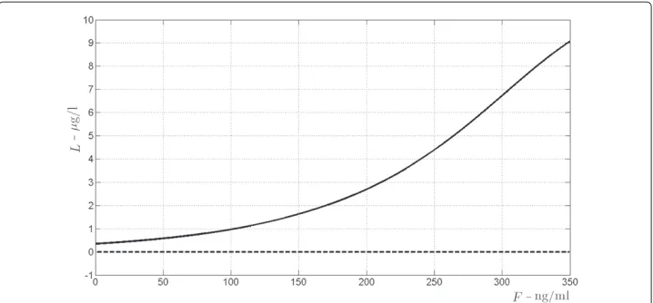
It turns out that there exists a unique triple of real positive solutions(S,L,Cl)for system (32), whose values are depicted in Figure 7 versus the drug concentrationF. It has to be stressed that this equilibrium point is locally asymptotically stable whatever the value of

F. Figures 8, 9, 10 refer to the bifurcation diagrams forS,LandClwith respect to the drug concentrationF.