A Polynomial Regression Analysis
Eleazar C. Nwogu
Department of Statistics
Federal University of Technology Owerri
Chigozie K. Acha
Department of Mathematics, Statistics and Computer Science
Michael Okpara University of Agriculture Umudike
Abstract
This paper discusses the age of birds at optimal production of egg. The objective is to determine the age at which birds are at their best in terms of production of eggs which may be relevant in improving the output of poultry farmers in egg production. To achieve this objective, secondary data on egg production (in grams per day) by age of birds (in weeks, from 18 to 87 weeks) between 2008 and 2010 were collected from poultry farm of the National Root Crop Research Institute (NRCRI), Umudike. This was analysed to determine the appropriate model for age-pattern of egg production among birds aged 18 to 87 weeks. Result of the analysis show that polynomial of order 3 describes the pattern in the egg production data well, but not adequately. The result also shows that the residuals from the fitted polynomial follow the pattern autoregressive process of order 1. Using the fitted model, it was observed that the age of birds at maximum production of eggs is about 44.36 weeks. The egg production corresponding to this age is about 12.14 grams per day. The birds were also found to be at their best, (in terms of egg production ) when they are aged between 34.5 weeks and 54.5 weeks, with egg production of at least 11.07 grams per day Hence, for optimal production of eggs, it is recommended that birds are not kept far beyond 54.5 weeks.
Keywords: Egg production, Polynomial Regression, Birds, Cubic model, Poultry product.
1. Introduction
Acha (2010) had emphasized the need for more efficient production of birds. In the same vein Sacra et al. (2008), Pollock (1997), Molenor et al. (2008) and Schmidt (2008) have stressed on the importance of verifying factors that are relevant to improved poultry production. Egg production, in particular and poultry farming, in general, are affected by many factors which includes feeding, water quality, housing and environmental conditions, temperature, management practices, the body weight of birds, bird strain, age of birds, poultry disease and disturbance [Banerjee (1998); Okereke and Nwogu (2010)]. Any poultry farmer desirous of improving his/her output must, therefore, take these factors into consideration. Many poultry farmers have been able to improve the quality of sanitation and environmental conditions; provide adequate feeding and vaccination for their birds. But bird strain and age of birds remain the factors necessary for improved quantity and quality of egg and poultry products in general that are yet to be controlled. In their study of correlates of eggshell thickness, Okereke and Nwogu (2010) observed that eggshell thickness is significantly associated with age of birds at lay. However, the study did not investigate the nature of this association.
The purpose of this study, therefore, is to determine the nature of the relationship between age of birds and egg production which may be utilized to improve production of egg. The essence is to determine the age range of birds at optimal production of egg that may help farmers to make informed decision on when to cull their birds.
The paper consists of five sections. Section 1 is the introduction, Section 2 presents the methodology of this study and Section 3 examines the need for transformation and choice of appropriate transformation for the study data. The choice of the appropriate regression equation of egg production on age of birds and estimation of the model parameters are discussed in Section 4, while Section 5 contains the summary, recommendation and conclusion.
2. Methodology
The data was analysed using the method of polynomial regression since age is the only independent variable appearing with various powers. The polynomial regression model is of the form
i X f
Yi i
e
(2.1), week ith the for where
ki p
0 k
k
i b X
X
f
(2.2)
i
Y is the egg production (in grams per day), Xi is the age of birds (in weeks), bk is the kth regression coefficient, b0 is intercept, p is the order of the polynomial and
e
iis theerror associated withY assumed to be uncorrelated and normally distributed with zero i mean and constant variance.
In some occasions, the residuals ( i
e
) may or may not satisfy some or all these conditions. Ifi
e
is completely random and normally distributed with constant variance, then the fitted model is said to describe the study data adequately. If not, the observed patterns of autocorrelation function (ACF) and partial autocorrelation function (PACF) may be used to identify and fit the appropriate probability model to the residuals in order to achieve adequate fit as recommended by Box et al. (1994). The selected probability model, (i.e. the Autoregressive- Moving average ARMA model) may be fitted using the Box – Jenkins procedure. For details of Box – Jenkins procedure see Box et al. (1994).In order to evaluate the study data for these assumptions, the normality assumption was investigated by examining the basic statistics of the data (including the mean, median and measures of skewness and kurtosis). Furthermore, the Box – Cox (1964) transformation procedure which jointly investigates the need for and determines the appropriate transformation was also adopted to check the normality assumption and stability of variances. For details of the Box – Cox transformation procedure see Akpanta and Iwueze (2007). However, as noted by Iwu (2009), when data is transformed, the original form of the data, as well as the unit of measure are altered.
The adequacy of the fitted model was also assessed using the JB statistic defined by Jarque and Bera (1980) as
22 2
1
24 n 6
n
JB (2.2)
0 2 4 6 8 10 12 14
0 2 4 6 8
3. Need for and Choice of appropriate Transformation of Egg production Data
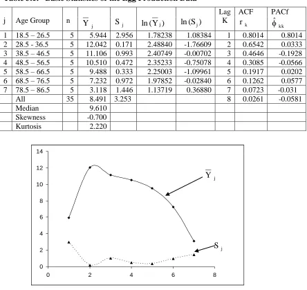
In order to gain more insight into the patterns of variation of trend and variance of the egg production data, the data was partitioned into seven equal parts. The overall and group basic statistics of the egg production data are shown in Table 3.1 while the graphs of the group means (Y ) and standard deviations (j Sj) are shown in Figure 3.1. As Table 3.1 shows, the overall mean (8.4914) is not equal to the median (9.610) as expected in a normal population. The measures of Skewness (1 0.700) and Kurtosis
( 2 0.780) also do not appear consistent with those of a normal population.
Table 3.1: Basic Statistics of the Egg Production Data
Y j
Sj
Figure 3.1: Graphs of the group means (Y ) and standard deviations (j Sj)
j Age Group n
j
Y Sj ln(Yj) ln(Sj)
Lag K
ACF
k
r
PACf
kk
ˆ
1 18.5 – 26.5 5 5.944 2.956 1.78238 1.08384 1 0.8014 0.8014
2 28.5 - 36.5 5 12.042 0.171 2.48840 -1.76609 2 0.6542 0.0333
3 38.5 – 46.5 5 11.106 0.993 2.40749 -0.00702 3 0.4646 -0.1928 4 48.5 – 56.5 5 10.510 0.472 2.35233 -0.75078 4 0.3085 -0.0566
5 58.5 – 66.5 5 9.488 0.333 2.25003 -1.09961 5 0.1917 0.0202
6 68.5 – 76.5 5 7.232 0.972 1.97852 -0.02840 6 0.1262 0.0577
7 78.5 – 86.5 5 3.118 1.446 1.13719 0.36880 7 0.0723 -0.031
All 35 8.491 3.253 8 0.0261 -0.0581
Median 9.610
Skewness -0.700
-3 -2 -1 0 1 2 3 4
0 10 20 30 40 50 60 70 80 90
0 2 4 6 8 10 12 14
0 5 10 15 20 25 30 35 40 45 50 55 60 65 70 75 80 85 90
-5 -4 -3 -2 -1 0 1 2 3 4 5
0 10 20 30 40 50 60 70 80 90
-10 -8 -6 -4 -2 0 2 4 6 8 10
0 10 20 30 40 50 60 70 80 90
The autocorrelation function (r ), shown in Table 3.1, indicates that the data are serially k correlated and not independent. Table 3.1 and Figure 3.1 also show that group standard deviations range from about 0.171 to about 2.956, indicating that the variance may not be constant. Thus, the basic statistics indicate that egg production data may not be independent, normally distributed and may not have constant variance and perhaps, require some transformation.
However, the slope (Y 1.35) of the regression equation of the logarithm of the group standard deviations on the logarithm of the group means (with an associated p-value of 0.100) is not significantly different from zero. This indicates that the data does not need any transformation.
4. Choice of appropriate model and estimation of model parameters
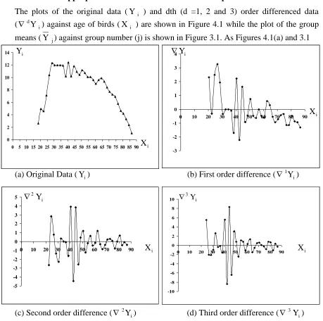
The plots of the original data (Yi ) and dth (d =1, 2 and 3) order differenced data (dYi) against age of birds (Xi ) are shown in Figure 4.1 while the plot of the group
means (Y ) against group number (j) is shown in Figure 3.1. As Figures 4.1(a) and 3.1j
i
Y Yi
Xi
Xi
(a) Original Data (Y ) (b) First order difference (i 1Yi)
2Yi i
3 Y
X i X i
(c) Second order difference (2Yi) (d) Third order difference (3Yi)
show, the curve which appears to describe the pattern in the study data may be a polynomial of order 2 or 3. The plots of the second and third order differenced series appear to oscillate about a line through zero, indicating that the differenced series may be stationary in mean. Thus, the choice of polynomials to be entertained lies between the quadratic and cubic curves. Since the quadratic is contained in the cubic equations only the cubic equation was fitted.
The fitted equation is
3i 2
i i
i 15.0711 1.4236X 0.0227X 0.0001X
X
fˆ (4.1)
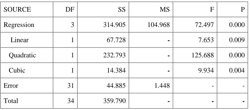
The analysis of variance for the fitted model is shown in Table 4.1. As Table 4.1 shows, the p-values associated with the regression coefficients indicate that the coefficients of all the terms in the model are significantly different from zero. Since the coefficient of the cubic term is significant it means that polynomial of order 3 in Equation (4.1) may be more appropriate to describe the pattern in the study data than the quadratic curve. The
value of 2
R for the fitted model is 87.5 percent, indicating that about 87.5 percent of the total variation in the egg production data is explained by its dependence on age of birds.
Table 4.1: Analysis of Variance for the fitted curve
SOURCE DF SS MS F P
Regression 3 314.905 104.968 72.497 0.000
Linear 1 67.728 - 7.653 0.009
Quadratic 1 232.793 - 125.688 0.000
Cubic 1 14.384 - 9.934 0.004
Error 31 44.885 1.448 - -
Total 34 359.790 - - -
The actual data (Yi) and the fitted (Yˆ ) values of egg production as well as the residuals i
are shown in Appendix A, while the plots of the actual (Yi) and the fitted (Yˆ ) values i
are shown in Figure 4.2. Appendix A and Figure 4.2 show that the fitted Equation appears to describe the pattern in the egg production data well, especially among birds aged 30.5 weeks and above.
0 50 100 150 200 250 300 350 400
0 5 10 15 20 25 30 35 40 45 50 55 60 65 70 75 80 85 90
Fitted
YˆiActual
Yi
Xi
Figure 4.2: Actual (Yi) and the fitted values (Yˆ ) of Egg production i
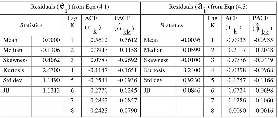
However, to assess the adequacy of the fitted model for the study data, the basic statistics, the autocorrelation function (ACF) and the partial autocorrelation function (PACF) of the residuals
i i Yˆ Y
i
e
(4.2)are calculated and shown in Table 4.2. When compared with the 95% confidence limits ( 2 n = 0.3381), the ACF of the residuals (
i
e
), shown in Table 4.2, appears not tocutoff, while the partial autocorrelation function (PACF) cuts off after lag 1. This implies
that the residuals ( i
e
) are not completely random and that the fitted model, fˆ
Xi in(4.1) does not describe the pattern in the study data adequately. Since the PACF ( kk ˆ
)
cuts after lag 1, the autoregressive process of order 1, AR(1),
i 1 i i
a
e
e
1 0
i i Yˆ Y
Table 4.2: Basic statistics of the residuals from fitted models
Residuals ( i
e
) from Eqn (4.1) Residuals ( ia
) from Eqn (4.3)Statistics Lag K ACF ( k r ) PACF ( kk ˆ
) Statistics
Lag K ACF ( k r ) PACF ( kk ˆ ) Mean 0.0000 1 0.5612 0.5612 Mean -0.0056 1 -0.0935 -0.0935
Median -0.1306 2 0.3943 0.1158 Median 0.0599 2 0.2117 0.2048
Skewness 0.4062 3 0.0787 -0.2692 Skewness -0.0100 3 -0.0776 -0.0449
Kurtosis 2.6700 4 -0.1147 -0.1651 Kurtosis 3.2400 4 -0.0398 -0.0968
Std dev 1.1490 5 -0.2541 -0.0936 Std dev 0.9230 5 -0.1257 -0.1166
JB 1.1213 6 -0.2770 -0.0245 JB 0.0846 6 -0.0724 -0.0698
7 -0.2862 -0.0857 7 -0.1286 -0.1060
8 -0.2423 -0.0790 8 0.0090 0.0016
is fitted tentatively to the residual series ( i
e
) and estimates of the parameter are shown in Table 4.3. Here,i
a
is the error associated, assumed uncorrelated and normally distributed with zero mean and constant variance. From Table 4.3 it is clear from the t-value that theTable 4.3: Final Estimates of Parameters
Type Coef Std Dev T
AR1 0.6142 0.1408 4.36
Constant -0.0435 0.1593 -0.27
constant (0) is not significantly different from zero, while the coefficient of AR(1) is
significant. Therefore, the final estimate of 1 in the model is 0.6116 and the fitted model is
i 1 i 0.6116
i
e
a
e
(4.4)The ACF and PACF associated with the residuals ( i
a
) shown in Table 4.2 indicate that the model in (4.4) describes the pattern ini
e
adequately since all of them lie within the 95% confidence interval ( 2 n = 0.3381).From Equations (4.1) and (4.4), the model which describes the pattern of egg production as a function of age of birds becomes
X ,
15.0711 1.4236X 0.0227X 0.0001X 0.6116 i 1fˆ
e
3ie
2 i i
i i (4.5)
where
i
e
is as defined in (4.3) andi
a
is a completely random and approximately normally distributed process with zero mean, standard deviation 0.9223,0.01
Hence, the age of birds at optimum production of eggs is about 44.36 weeks with
X 12.14fˆ i . In fact grams per day. In fact, the birds appear to be in their best, in
terms of egg production, when they are in the age range 34.5 to54.5 weeks. In this age range, their output is at least 11.07 grams per day. Therefore, for optimal production of eggs, it is recommended birds are not kept beyond 54.5 weeks of age.
5. Summary, Recommendation and Conclusion
The main objective of this study is to determine the age of birds at optimal production of eggs which may be relevant in improving the output of poultry farmers and poultry products. The relevance of this lies in the fact that it will enable the poultry farmers to know the age of birds that produce the maximum amount of eggs and how long to keep them. To achieve this, the data on egg production (in grams per day) by age of birds collected from the poultry farm of N.R.C.R.I., Umudike was first evaluated for the assumptions of regression analysis. Thereafter, the appropriate model, which adequately describes the observed pattern of egg production by age of birds was identified and fitted.
The result of the analysis shows that, although the assumptions are not completely satisfied, no transformation was suggested. Polynomial of order three was found to describe the pattern in observed data well, though not adequately. Using the pattern of the ACF and PACF of the residuals from the fitted polynomial, the autoregressive process of order 1 was identified and fitted to the residuals. The fitted model shows that the age of the birds at maximum is about 44.36weeks. The corresponding egg production at this is about 12.14 grams per day. The birds were also found to be at their best, in terms of production of eggs when they are aged 34.5 weeks to 54.5 weeks, when their output is at least 11.07grams. per day
Hence, for optimal production of eggs, it is recommended that birds are not kept beyond 54.5 weeks.
References
1. Acha, C.K. (2010). Impact of Housing and Age of Birds on Egg production.
International Journal of Numerical Mathematics, 5(2), 275 – 298.
2. Akpanta A.C and Iwueze, I. S. (2007). On the effect of logarithmic transformation on Multiplicative time series model. Ph.D. thesis Abia State University, Uturu, Nigeria.
3. Banerjee, G.C. (1998). A text Book of Animal Husbandary, Eight Edition, Oxford
and IBH Publishing Co. Pvt, New Delhi.
4. Bartlett, M.S (1947). The use of transformation. Biometric Bulletin, 3, 36-52.
5. Bland, J.M. and Attman, J.M. (1996). Statistics Notes, Transforming data. British Medical Journal, London, 312, 770.
7. Box, G.E.P., Jenkins G.M. and Reinsel, G.C. (1994). Time series Analysis; forecasting and control. Prentice-Hall, New Jersey.
8. Iwu H.C. (2009). Transformation and Decomposition of Multiplicative time
Series Model, Ph.D Thesis Abia State University, Uturu Nigeria.
9. Jarque, O.M. and Bera, A.R. (1980). Efficient tests of normality,
homoscedasticity and serial independence of regression residuals. Econometrics Letters, 6(3), 255 – 259.
10. Okereke, O. E. and Nwogu, E. C. (2010). Correlates of Eggshell thickness. Global Journal of Pure and Applied Sciences, 16(2), 261 – 268.
11. Molenar, R, Reijrink I.A.M: Merjerhof, R. and Van Den Brand, H. (2008). Relationship between Hatchiling Length and weight on later productive performance of Broilers. World’s Poultry Science Journal, 64, 599 – 604.
12. Pollock, D. L. (1997). Maximizing Yield. Poultry Science 76, 1131 – 1133.
13. Sacra, M., Boga, S and Yamak, U. S. (2008). Effects of Space Allowance on Egg
Yield, Egg Quality and Plumage Condition of laying Hens in Battery Cage. Czech Journal of Animal Science 8(53), 116 – 121.
14. Schmidt, G. S. (2008). Evaluation of Technical and Economic Impacts of High –
Appendix A: Actual (Yi), the fitted values (Yˆi) of Egg production and Residuals (
i
e
) from the fitted model (4.1)i Xi Yi Yˆi
e
i1 18.5 2.63 4.1117 -1.4817
2 20.5 4.95 5.4122 -0.4622
3 22.5 4.62 6.5796 -1.9596
4 24.5 7.12 7.6189 -0.4989
5 26.5 10.40 8.5346 1.8654
6 28.5 12.34 9.3317 3.0083
7 30.5 11.99 10.015 1.9750
8 32.5 11.99 10.589 1.4010
9 34.5 11.99 11.0588 0.9312
10 36.5 11.90 11.4289 0.4711
11 38.5 10.19 11.7043 -1.5143
12 40.5 12.41 11.8896 0.5204
13 42.5 10.19 11.9897 -1.7997
14 44.5 11.83 12.0093 -0.1793
15 46.5 10.91 11.9532 -1.0432
16 48.5 10.45 11.8261 -1.3761
17 50.5 11.20 11.633 -0.4330
18 52.5 10.73 11.3784 -0.6484
19 54.5 10.09 11.0672 -0.9772
20 56.5 10.08 10.7042 -0.6242
21 58.5 9.61 10.2941 -0.6841
22 60.5 9.00 9.8418 -0.8418
23 62.5 9.59 9.3519 0.2381
24 64.5 9.89 8.8293 1.0607
25 66.5 9.35 8.2787 1.0713
26 68.5 8.42 7.7050 0.7150
27 70.5 7.71 7.1128 0.5972
28 72.5 7.29 6.5070 0.7830
29 74.5 6.94 5.8924 1.0476
30 76.5 5.80 5.2736 0.5264
31 78.5 4.66 4.6556 0.0044
32 80.5 4.19 4.0430 0.1470
33 82.5 3.31 3.4406 -0.1306
34 84.5 2.37 2.8532 -0.4832