Flow field mapping in data rack model

Flow field mapping in data rack model

L. Manoch1, J. Matě_cha1_{, and P. Pohan}2

1_{CTU in Prague, Department of Fluid Mechanics and Thermodynamics, Technická 4, Praha, Czech Republic} 2_{Conteg, spol. s r.o., Na Vítězné pláni 1719/4, Praha, Czech Republic}

Abstract. The main objective of this study was to map the flow field inside the data rack model, fitted with three 1U server models. The server model is based on the common four-processor 1U server. The main dimensions of the data rack model geometry are taken fully from the real geometry. Only the model was simplified with respect to the greatest possibility in the experimental measurements. The flow field mapping was carried out both experimentally and numerically. PIV (Particle Image Velocimetry) method was used for the experimental flow field mapping, when the flow field has been mapped for defined regions within the 2D/3D data rack model. Ansys CFX and OpenFOAM software were used for the numerical solution. Boundary conditions for numerical model were based on data obtained from experimental measurement of velocity profile at the output of the server mockup. This velocity profile was used as the input boundary condition in the calculation. In order to achieve greater consistency of the numerical model with experimental data, the numerical model was modified with regard to the results of experimental measurements. Results from the experimental and numerical measurements were compared and the areas of disparateness were identified. In further steps the obtained proven numerical model will be utilized for the real geometry of data racks and data.

1 Introduction

The paper aims to build on existing work in investigation of flow in data racks. Several approaches were designed and verified within the previous research allowing for identification of the flow field within the data rack. Evaluation of pre-defined criteria, which were based on general assumptions regarding the evaluation of a flow field in a given geometry, lead to proposing a methodology of identification of the flow field and the temperature field. This methodology includes both experimental and numerical part of solution and evaluation.

2 Model

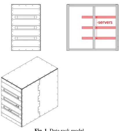
Because of considerable complexity of preparation and adjustments of original data racks for experimental measurement, a data rack model (figure 1) was designed and built within the new methodology that preserves the original features and dimensions of real data rack. However, the data rack internal layout and geometry was considerably simplified. The data rack model was also designed with regard to the need to simulate different variations of compilations based on the real data rack.

Fig. 1. Data rack model.

Dimensions of the model itself are based on data rack capable of holding 19 1U servers. For this case, the data rack model was fitted with only three 1U models of servers that were used in previous measurements. This model by its design is based on real 1U server fitted with four sockets for CPU. Eight modules for installation of RAM were subsequently assigned to each CPU. The reason for using a server model instead of real four-C

Owned by the authors, published by EDP Sciences, 2013

This is an Open Access article distributed under the terms of the Creative Commons Attribution License 2 0 , which . permits unrestricted use, distributi

socket 1U server is that we were able to regulate both the performance of fans (channel C) and individual heat sources representing the aforementioned CPU (channel A) and RAM (channel B). Regulation of individual channels is possible in the range of the order of units of percents up to 100%. Within this paper, all 2D PIV results were measured and evaluated for 100% performance of the fans. The other two channels for CPU and RAM were set to the lowest value. Their influence was not considered within the evaluation.

All data rack walls were made of transparent material. This solution enables the identification of the flow field even in places where the identification in the real data rack would be completely impossible. The front of the data rack model was designed in order to simulate possible recirculation within the data rack body, which happens to be the a very undesirable phenomenon with regard to cooling of servers.

One of the desired results is the quantification of flows within the recirculation zone. Another modification, as opposed to the real data rack, is a circular hole in the bottom of data rack model due to power supply and management of server models. The hole diameter was chosen as the smallest possible due to the power connectors.

3 Experimental measurements

A 2D PIV method was used for identification of the flow field. The flow field was investigated for two cuts located in the plane parallel to the main plane of data rack model symmetry. The cuts were located with respect to the comparison with numerical simulation inside and outside the data rack. The reason for the location was the investigation of the nature of the flow field for highly geometrically limited area, for interior of the data rack model and for free area defined by free space in the data rack outlet.

A measurement setup consisting of three main blocks was designed and built for using the 2D PIV (figure 2) method to identify the flow. Each of the main blocks can be further divided into subparts. For this case, following blocks were considered:

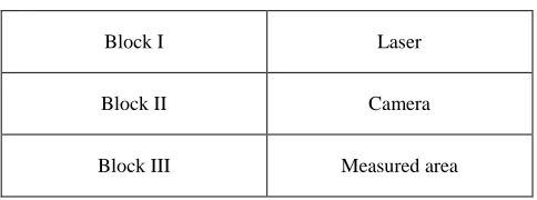
Table 1. 2D PIV assembly blocks.

Block I Laser

Block II Camera

Block III Measured area

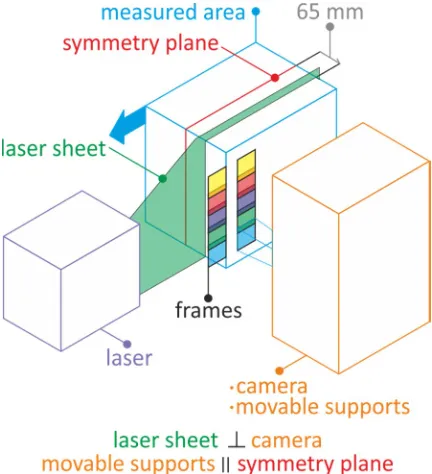
Interrelationships between individual blocks (figure 3) helped to achieve optimum repeatability of the measurement. These relationships were important also in terms of measuring the flow fields because the flow fields were measured separately but within the same plane.

As already mentioned above, the measurement plane was parallel to the data rack main symmetry plane. However, it was shifted by 65 mm in the positive

direction of the y-axis. The reason for shifting was the fact that the power supply and management of individual servers were located in the symmetry plane and the servers in the area generated a minimum mass flow rate. Under this assumption, secondary flow was expected do develop in this area.

3.1 2D PIV

For 2D PIV method, a laser (BSL produced by QUANTEL company) with a performance of 220 mJ in pulse and a frequency of 10 Hz was used for illumination of the measurement plane. It was necessary to adjust the position of the laser sheet during the measurement so that the measured area was continuously illuminated by necessary intensity and the signal degradation was avoided.

Fig. 2. 2D PIV experiment configuration.

A camera with 2048 ∙ 2048, 12-bit resolution was used for recording of the image. The camera was placed perpendicular to the laser sheet. A positioning device was used for the camera movement in the plane parallel to the laser sheet. In the positive direction of the z-axis (data rack height), the positioning device was controlled via PC and the movement was provided by stepping motor. In the direction of x-axis (data rack length), both in positive and negative direction, the movement of the positioning device was carried out by ball screw with manual feed and a digital readout distance.

For a defined measurement area, a square sector was chosen in the required plane with an edge 120 mm long, which measured the whole data rack height with a 20% overlap in the positive direction of the z-axis.

was significantly better than from the fog generator produced by SAFEX company.

All PIV setup and information about measurement were acquired from [1].

Fig. 3. 2D PIV assembly block configuration.

3.2 Outlet velocity profile

With the help of 2D network (figure 4), a velocity field was mapped for the rectangular outlet of data rack measuring 353 ∙680 _{mm. The field was mapped with the} help of propeller anemometer for all inner nodes of 2D network. The edge length when dividing the horizontal dimension of the 353 mm long rectangular output into 4 parts was chosen as the major dimension of the network element. The above mentioned dimension, according to the definition, was equal to 88.25 mm. For the other dimension, the network was divided into the nearest whole number of parts where the edge length was related to the main dimension of the 2D network element. The resultant 2D network had dimensions of 4 ∙ 7. The resulting dimension of the network also shows the total number of mapped points, which in this case was equal to 18 points.

For creation of a real 2D network a thread probe was used whose diameter was completely negligible in relation to other dimensions of the output. Considering the above, the output velocity field was affected minimally.

The flow field was measured with the help of 2D PIV method only for maximum performance of the server fans (channel C). The remaining two channels for CPU (channel A) and RAM (channel B) were set to the lowest possible value.

A 2D velocity field on the data rack output was measured for 5 different performances on the server fans. These were 20%, 40%, 60%, 80% a 100% of the

performance. The mass flow rates were then generated from those flow fields

Fig. 4. 2D grid scheme.

4 Numerical simulation

The model designed for the experimental part was projected with regard to the use of this model geometry for numerical simulation. Within the geometry of the data rack model for numerical simulation, the model was complemented by connecting and supporting members providing the proper functionality of the whole at experimental measurement. The members that could be expected to affect the flow field were incorporated into the model geometry. Those were the supports of individual servers and connecting corner parts of the entire inner construction of the data rack. They were added to the model to the outlets of individual servers representing the inlet to the computational area, the area for local softening of the calculation mesh. In the last step, the boundary area was defined.

The entire computational mesh was created in the Beta ANSA program based on the imported geometry and data rack area. The computational mesh contained only elements of four-wall type, namely the total number approximately of 13 millions elements. All boundary conditions were defined within the process of creating the computational mesh.

Two solvers were used for numerical simulation. These were Ansys CFX v14 and OpenFOAM v2.1.1. The same above-mentioned computational mesh was used for both solvers. The same turbulence model was used, namely the two-equation SST k-omega turbulence model (Menter).

computational mesh. The boundary condition for the OpenFOAM was defined as a constant velocity vector where the magnitude of the velocity vector was calculated from the mass flow rate of the measured velocity field.

Fig. 5. Velocity inlet profile for CFD simulation.

5 Evaluation

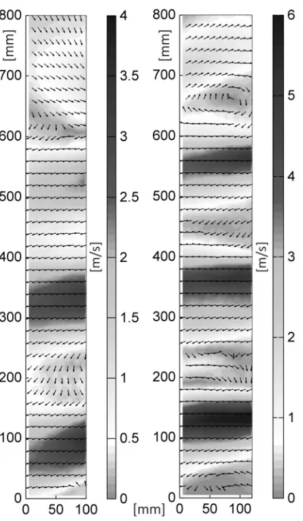
Individual flow patterns were compared in the investigated areas (figure 7). From the results we can see, that CFD model do not fit to experimental data. There was achieved some similarity in the flow field pattern but maximum value of velocity in the measured planes was higher about 30 percent for experimental measurement (figure 6) than for CFD (figure 8).

Fig. 6. Velocity fields [m/s] from experiment measurement

Fig. 7. Defined examined areas

Fig. 9. Experimental velocity [m/s] samples from 2D grid on

data rack outlet.

Velocity fields from 2D grid (figure 9) on data rack outlet for five different performances were evaluated.

6 Conclusion

From the results mentioned above it is clear that a used turbulent model under the given boundary conditions can’t describe the flow field. 2D grid at the output of the data rack model does not have sufficient density for the determination and comparison of mass flow.

From this point of view the different turbulent model must be used for flow field description. Also the finer grid has to be used for suitable results.

For the future work more 2D and 3D PIV measurement will be done. Also some continuous visualization of flow field across whole data rack and temperature fields are in plans. All this will support finding suitable CFD model.

Acknowledgment

Project (TA01010184 / Research and development solutions data racks, cooling and transport systems for data centers) is / was solved with the financial support of TA Č_R.

References

1.

2.